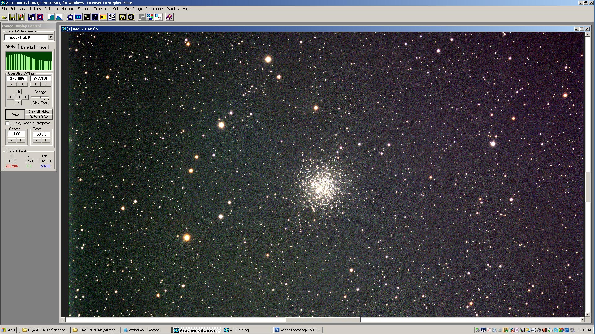
Figure 1. Initial appearance of the FITS RGB color composite image of NGC 5897 displayed in AIP4WinV2.
USING PHOTOSHOP TO CONTRAST-STRETCH 16-BIT RGB IMAGES TO PRODUCE IMPROVED 8-BIT RGB IMAGES
(June 2015)
Okay, so you've carefully applied basic image processing procedures like those described on this website to align, calibrate (for atmospheric transmissivity), and correct (for camera and filter characteristics) your astro-images and to remove imaging system-related artifacts (thermal noise, hot pixels, vignetting and dust "doughnuts"). You've saved it as a FITS RGB color composite image. It should be a realistic representation of what the object should look like. So, when you display it in your image processing software, you get something like Figure 1. Yes, you can see the object (in this case, the globular cluster NGC 5897) in the image, but it looks terrible! The backgoung is grainy and not "black" like the sky should be, and maybe even shows traces of a slight gradient in the color. The stars are mostly white dots, with the brightest showing a strongly saturated core with just a hint of color around them. The overall image is flat, muddy and uninteresting. So, what happened to your carefully processed image?
Figure 1. Initial appearance of the FITS RGB color composite image of NGC 5897 displayed in AIP4WinV2.
First of all, there likely is nothing wrong with your processing, as is the case with the image in Figure 1. The appearance of the image in Figure 1 is the result of trying to display the distribution of image pixel values making up the FITS RGB image on a device (your computer monitor) that has a limited display capability. We can start to get a grasp of this problem by looking at Figure 2. This figure shows the histogram of pixels values for the image in Figure 1, with the rangle of pixels values displayed on the x-axis and the number of image pixels with a given pixel value displayed on the y-axis. Note that the y-axis is constructed using a logarithmic scale— the seven sets of horizontal lines on the green background represent seven orders of magnitude (each a power of 10). So, while the lowest set of horizontal lines represents pixel numbers from 1 to 10 pixels, the upper set of horizontal lines represents pixel numbers from 1 million to 10 million pixels. In this type of FITS image, pixel values are stored as signed 32-bit floating point numbers, so you can see that the individual pixel values can span a tremendous range. For the image in Figure 1, the lowest pixel value is 0, while the highest pixel value is 91825.7. Looking at the histogram in Figure 2, it is obvious that the pixel values are not evenly distributed over this range. Of the 8,328,303 pixels in the image, the vast majority of them are concentrated on the low end of the range. This type of distribution is typical of astronomical images, where most of the image contains "empty space" between stars or extended objects with very low surface brightness (like nebulas or galaxies) compared to stars.
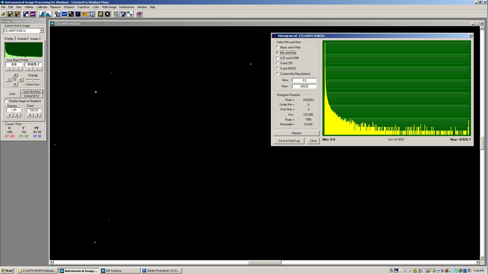
Figure 2. Histogram of the pixel values of the image of NGC 5897 from Figure 1.
So, how does this distribution of pixel values give rise to the problem in desplaying the image? Standard computer monitors are 8-bit display devices. This means that the range of brightness values in each of the red, green and blue color channels of the image will be divided up into 256 steps. In the displayed image, the lowest step (0) will be displayed as black, while the highest step (255) will be displayed as white (or, for the three color channels, saturated red, green, or blue). The intermediate steps between 0 and 255 will be assigned values that increase linearly in brightness from black to white. So, if we wanted to display the entire range of pixel values in the histogram from Figure 2, we would divide the range (0 to 91825.7) into 256 steps. Thus, the lowest step in the displayed image, which would be displayed as black, would include pixel values from 0 to approximately 358.7 (i.e., 91825.7/256). Unfortunately, practically all the pixels in the histogram representing the image of NGC 5897 would fall into this first step, and thus would be displayed as black. The result is shown in the image displayed behind the histogram in Figure 2— the image is almost entirely black, with only a few bright stars having pixel values great enough (i.e., greater than 358.7) to get them out of the lowest step in the displayed image. Notice that the cluster in the image doesn't show up at all. So, for most astronomical images, this approach is not going to work.
A common approach to get around this problem is to let the display range (0 to 255) represent only a subset of the entire range of pixel values in the image. For example, instead of letting the lowest display step (0) start at zero, it could start at a greater pixel value. Similarly, instead of letting the highest display step (255) end at the greatest pixel value, it could end at a lower pixel value. Commonly, the new starting and ending values for the range of displayed values is determined as fractions of the total number of pixels in the image. For example, we could establish that the lowest display value (0) corresponds to the pixel value at which 1% of the pixels have lower values. We could also establish that the highest display value (255) corresponds to the pixel value at which 0.5% of the pixels have greater values. For the histogram in Figure 2, this new low pixel value would be 270.886, while the new high value would be 421.480. So now, all pixels in the displayed image with pixel values less than or equal to 270.886 will be displayed as black, while all pixels in the displayed image with pixel values greater than or equal to 421.480 will be displayed as white. Thus, we have clipped off the lower and upper ends of the old histogram. Between these new bounds, displayed pixels will be assigned values that increase linearly in brightness from black to white, as before. But now, we have "re-mapped" the range of displayed values to only a portion of the original distribution. The result is shown in Figure 3.
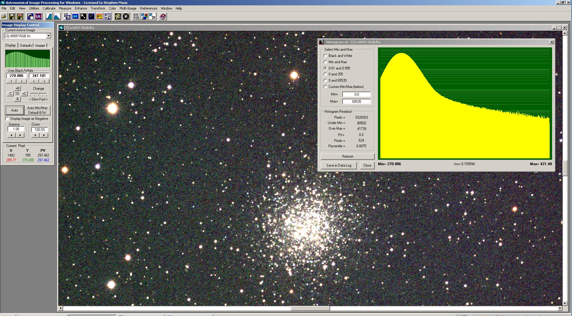
Figure 3. Re-mapped histogram of the pixel values and the resulting displayed image of NGC 5897.
In Figure 3, the new histogram shows a more uniform distribution of pixels over the range of pixel values. In the displayed image behind the histogram, the cluster and neighboring stars are now visible. In fact, this is the same as the displayed image in Figure 1, since this approach to re-mapping the histogram is the default display procedure used in AIP4WinV2. Again, we're probably not going to be completely satisfied with this version of the displayed image. However, we can do a little "fine-tuning" of the bounds of the histogram. As shown in Figure 4, we can use the controls in the Image Display Control box (on the left side of the screen display) to manually increase the lower bound from 270.886 to 293.790 and decrease the upper bound from 421.480 to 396.738. This action results in a nice, dark background in the displayed image along with sharply defined stars. If we're satisfied with this version of the image, we can save it as an 8-bit JPEG image file that we could post on the Internet. It's important to note that all these display manipulations have only affected the displayed image and have not changed anything in the original FITS image file.
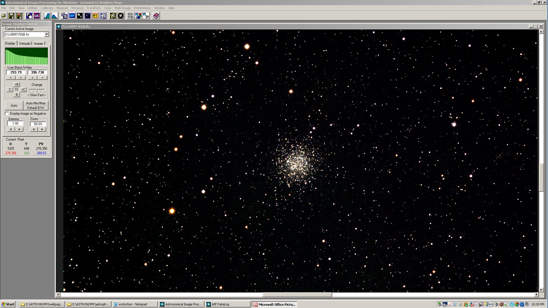
Figure 4. Displayed image of NGC 5897 after additional manual "fine-tuning" of the histogram bounds (compare with Figure 1).
While the image in Figure 4 is okay, it's not a really good representation of the imaged object. The stars are mostly white dots, except for some of the brighter ones that show a thin halo of color around a large saturated (white) core. The image lacks a feeling of depth, and almost resembes a black-and-white image. This is primarily because our choice for the upper bound for the histogram results in most of the pixels representing stars to fall into the highest display level (255) and thus be displayed as white.
We could continue to "fine-tune" the histogram bounds, but it won't improve the displayed image much. What we need is another approach for manipulating the huge range of pixel values in the original FITS RGB image to get it into a form that can be adequately accommodated by the 0-255 range of displayed image values. A potential solution is to "stretch" the range of pixel values in the original image to decrease the contrast between the brightest and dimmest pixels in the image. Then, when we divide this stretched range of pixel values into 256 steps, more of the original range in relative brightnesses can be contained within the 256 display steps between black and white.
There are a number of procedures that can be found in image processing software like AIP4WinV2 or Maxim DL to do this. They are usually called "contrast stretching" or "histogram specification" routines, since they work on the shape and not just the bounds of the histogram. In these routines, you usually pick a mathematical function, like a logarithmic curve or a gamma function, from a list of choices to convert each pixel value along the x-axis of the histogram into a new pixel value that hopefully will have the overall effect of reducing the contrast between the brightest and dimmest pixels in the image. This approach is a whole separate topic in image processing, and I won't go into its theory and details here. For the theory and details, see Section 13 ("Point Operations") in "The Handbook of Astronomical Image Processing" by Richard Berry and James Burnell (Willmann-Bell Publishers, Richmond, VA, 2009). In using these routines, you specify certain characteristics of the curve that affect its shape— you usually see the results in a preview window that contains a small portion of the entire image. If you like the effect, you can apply it to the entire image. If you don't like what this does to the displayed image, you can go back and undo the previous effect and fiddle with the curve some more until you evetually get through trial-and-error something you really like. Or maybe not. I'm not really satisfied with these contrast-stretching routines in the software packages I've worked with. You're limited in how you can manipulate the curve shape. Also, it's difficult to see in real-time how changing the curve is affecting the displayed image, except through the small preview window. There needs to be a better way of doing this histogram manipulation.
This is where Photoshop comes in. Photoshop is the premier digital image photo-editing software package. I don't think of Photoshop as "image processing" software like AIP4WinV2 or Maxim DL because it is not concerned with the quantitative aspects of the image data but rather the qualitative aspects of the displayed image, i.e., does the displayed image "look good"? This is actually fine for our purpose, since we've already insured that the quantitative aspects of the image are correct through our previous image processing procedures (image alignment, calibration, etc.). Photoshop is great for manipulating the appearance of a displayed image because it contains a lot of very flexible tools to do this and the effects of each step in using a tool can be seen in real-time in the entire displayed image. In the remainder of this section, I will demonstrate the use of a procedure in Photoshop for contrast-stretching images that almost always results in nice-looking images of astronomical objects, including star clusters, nebulas and galaxies. Note that, in contrast to the basic image processing procedures that I've described in other places on this website, the steps in this image manipulation procedure are not "cast in stone" and can be modified as you go through the process. The good thing is, even if you mess up the displayed image, you haven't affected the original image data.
The first step in the procedure is to get the image into a form that can be used in Photoshop. There are Photoshop plug-ins that allow the software to directly read FITS image files. I find it easy just to convert the FITS color composite image created in my image processing software into a 16-bit TIFF file (most image processing software packages like AIP4WinV2 will do this conversion). TIFF files are the standard graphic arts image format used in photo-editing software packages like Photoshop. Except for the very earlierst versions of Photoshop, most versions are set up to handle 16-bit TIFF files. I'm currently using Photoshop CS3.
Figure 5 shows the result of dragging and dropping the TIFF file representing the image in Figure 1 into Photoshop (your screen display may look somewhat different depending on your version of Photoshop and how you've got it set up). Again, the displayed image looks almost completely dark except for a few bright stars, as in Figure 2. This is because the default display method in Photoshop for these types of image files is the same as that used by AIP4WinV2 in Figure 2. By opening the "Levels" tool under "Adjustments" in the drop-down menu under "Image" in the Toolbar, you can see the histogram of the image data (in the "Input Levels" display) and verify that the lowest pixel value is displayed as black while the greatest pixel value is displayed as white (in the "Output Levels" display). This is shown in Figure 6.
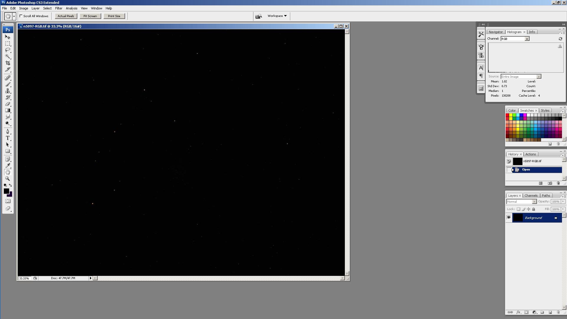
Figure 5. The TIFF version of the original RGB color composite image representing NGC 5897 displayed in Photoshop CS3.

Figure 6. Using the "Levels" tool in Photoshop to display the mapping of the image histogram to the range of displayed values between black and white.
To start the contrast-stretching procedure, bring up the "Curves" display under "Adjustments" in the drop-down menu under "Image" in the Photoshop Toolbar (Figure 7). Before making any changes to the image, be sure that "RGB" is selected from the "Channel" drop-down menu. All changes that you make must be applied equally to all three colors channels— otherwise, the color balance in the image will be messed up. The main part of the "Curves" display is the graph that shows the relationship between the starting distribution of pixel values (the x-axis, labelled "Input") and the modified distribution of pixel values (the y-axis, labelled "Output"). Figure 7 shows the situation before we have made any modifications, so the diagonal line in the graph shows that there is a 1:1 relationship between the input and output distributions. It will be through changes in this relationship that we will contrast-stretch the image data. The graph in the "Curves" display also shows the histogram of the starting distribution of pixel values. However, at this stage in the process, the pixel values so concentrated along the low end of the distribution (see the "Levels" display in Figure 6) that it doesn't even show up along the left edge of the graph. This will change as we proceed through our process.

Figure 7. Using the "Curves" display in Photoshop to visualize the relationship between displayed image inputs and outputs.
The first step in our stretching process is to get rid of a large portion of the upper end of the starting pixel distribution. Referring to the histogram in Figure 6, we can see that there is very little pixel information in the upper portion of the histogram— just pixel values for a few of the brightest stars. To "clip" this portion of the histogram off, use the white slider marker initially located at the right end of the x-axis in the "Curves" display. Grab it with the cursor and slide it to the left along the x-axis. As you're doing this, watch the displayed image. As you slide the marker to the left, a few more stars will start to "peek out" in the image. Still, moving it 3/4 of the way toward the left end of the x-axis (as shown in Figure 8) only changes the displayed image a little. With the slider marker in this position, every pixel in the displayed image with values at or above 1/4 of the range in the original distribution will be displayed as white. Go ahead and save this modification by clicking the "OK" button in the "Curves" display. When you do so, the modifications to the displayed image will be saved and the "Curves" display will disappear.
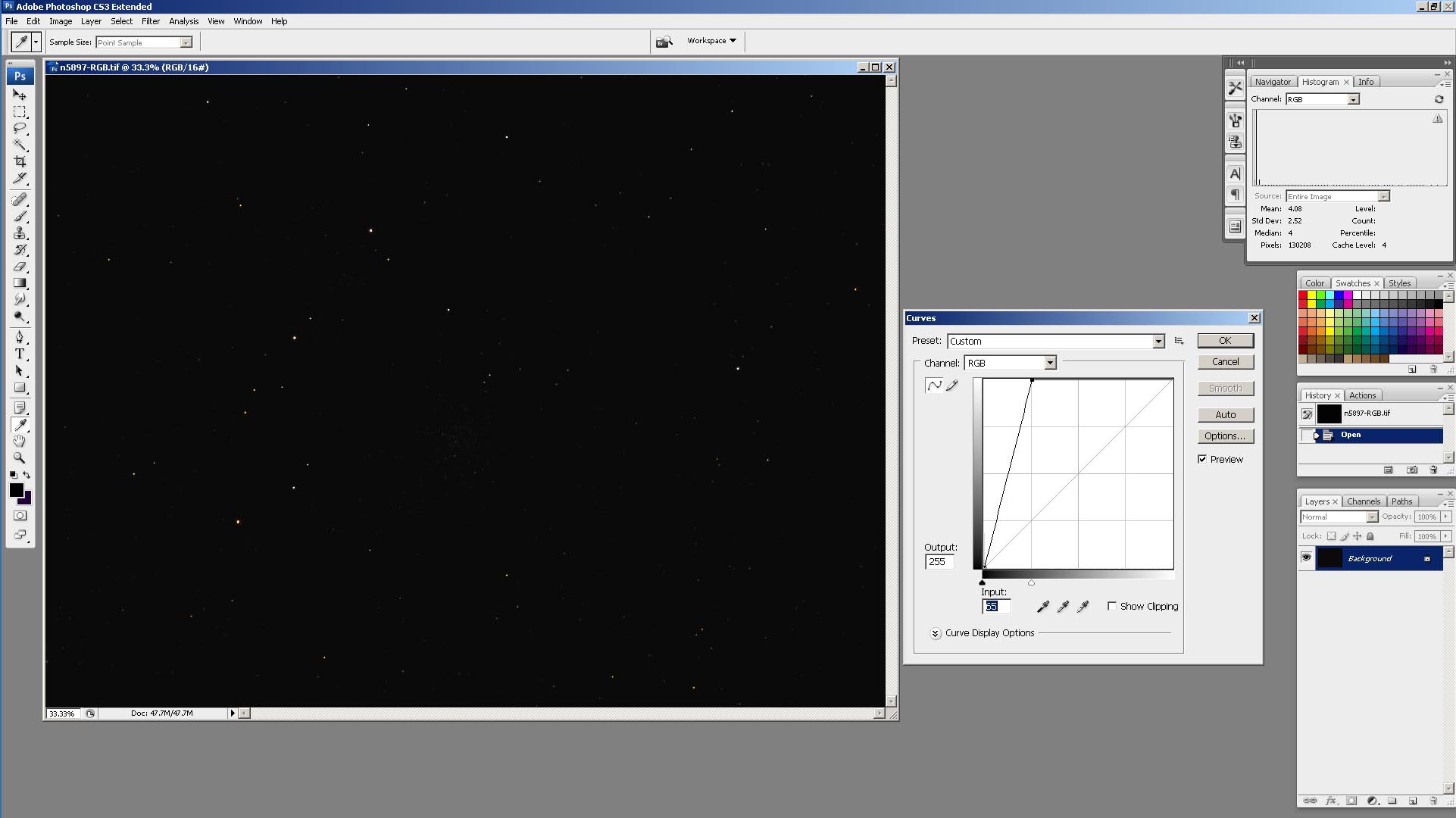
Figure 8. Changing the upper bound of the starting (input) pixel distribution.
As you will see, this approach to contrast-stretching is an iterative process. For the next step, open again the "Curves" display. It won't look much different from the previous version, but recognize that now the right end of the input distribution on the x-axis represents the point that used to be only 1/4 of the way between the distribution bounds in the original histogram. We've stretched the pixel data in what used to be the first 1/4 of the distribution over the entire range from black to white. So, our "output" from the previous step in the process will be the "input" for the current step. What we will start doing is modifying the shape of the relationship between "input" and "output" pixel values (initially the diagonal line in the graph) in a manner that increases the low values while holding the high values at about the same. In doing so, we will be decreasing the contrast between the brighest and dimmest pixels in the displayed image. If we do this carefully, we will be able after a number of iterations to produce a distribution of pixel values in the displayed image that will allow most of them to be accomodated by the 0-255 display range, thereby minimizing pixel saturation while maintaining the proper overall variations in the brightness of the astronomical objects in the image.
Our first attempt at modifying the shape of the input/output relationship is shown in Figure 9. To do this, we placed the cursor on the initially diagonal line in the graph at about 1/8 of the way from the left edge of the x-axis, held down the left mouse button, and "pulled" the curve upward. When we release the mouse button, a "point" will be left on the new form of the input/output relationship where we had "grabbed" it with the cursor. The shape of the new curve will increase the "output" values of the image pixels. Unfortunatey, this action will produce a curve that increases all the "output" pixel values over the entire range of the distribution. Recall that we only want to increase the values of the dimmer pixels while holding the brighter pixels at about the same values. To do this, use the cursor to again "grab" the curve, this time at around 2/3 of the way from the left to the right end of the x-axis. While holding down the mouse key, "pull" the curve down so that the upper portion of it again approximates a diagonal line. The resulting curve shape is shown in Figure 9. Looking at the displayed image, it doesn't look like it changed much. That's okay— this is a slow process. Go ahead and save this modification by clicking the "OK" button in the "Curves" display.
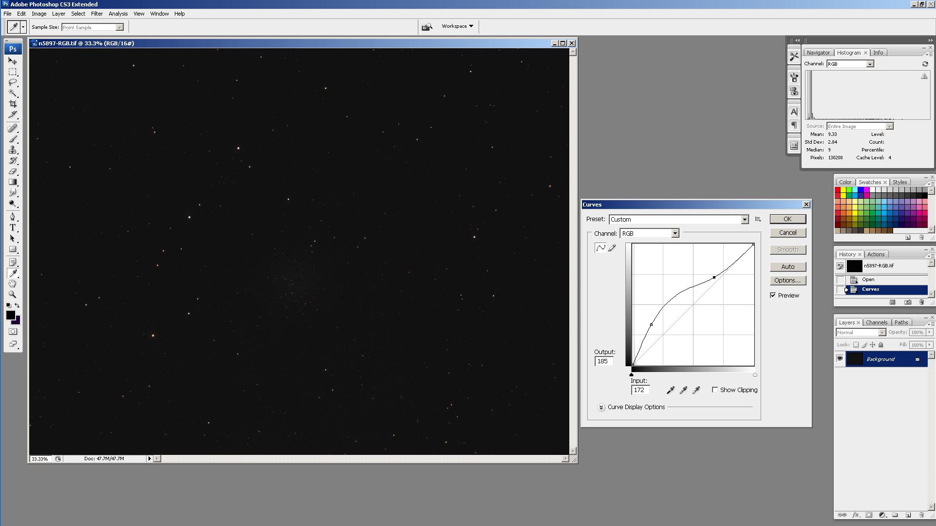
Figure 9. The first attempt at modifying the input/output relationship for the distribution of pixel values in the displayed image.
The next iteration is shown in Figure 10. But note that, this time when we open the "Curves" display, we can now see the histogram of the distribution (in light gray) near the left side of the graph. We make the same change to the shape of the input/output relationship as we did before. After we make this change, we can see more stars in the displayed image, including some stars in the globular cluster. Again, save this modification by clicking the "OK" button in the "Curves" display.
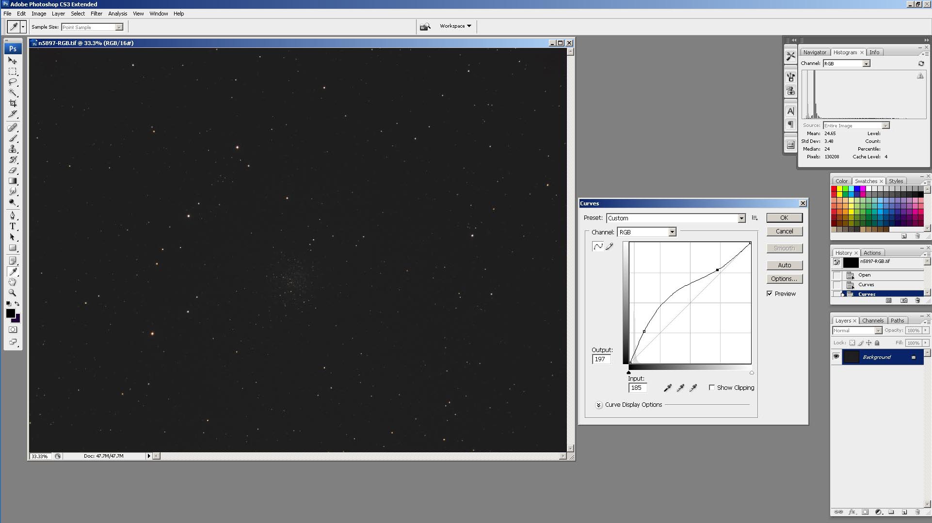
Figure 10. The second iteration in modifying the input/output relationship for the distribution of pixel values in the displayed image.
The third iteration of the process is shown in Figure 11. Note that the histogram of the pixel value distribution has gotten wider and has moved more to the right in the graph. When we perform our modification of the input/output relationship, we see a further increase in the number os stars in the displayed image. But, we also notice that the "empty" space between the stars is not black any more, but a dark gray. This is because we have now moved the histogram so far to the right that the pixel values between it and the left edge of the x-axis are no longer represented by "black". We will fix this in the next iteration. Go ahead and save this modification by clicking the "OK" button in the "Curves" display.
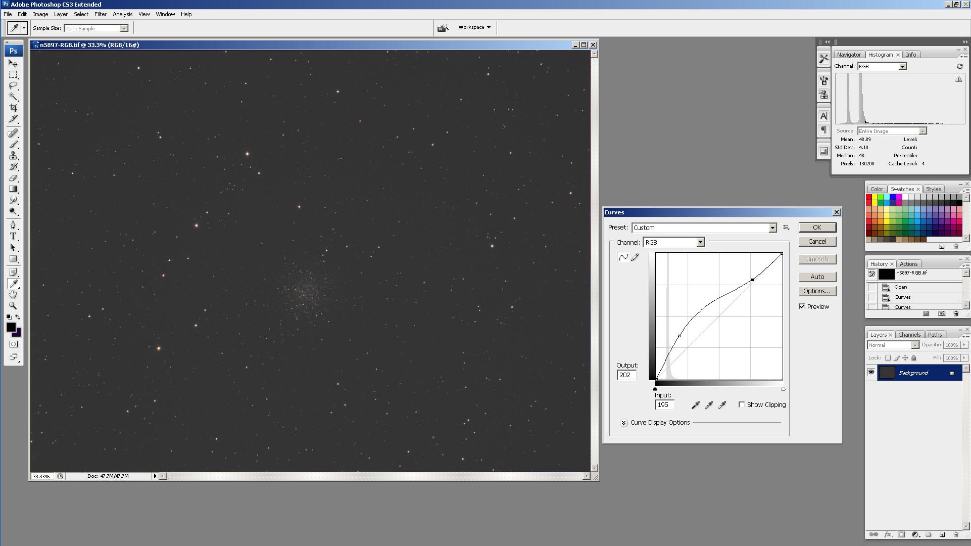
Figure 11. The third iteration in modifying the input/output relationship for the distribution of pixel values in the displayed image.
The pixel values between the left end of the x-axis and the histogram are "nothing" and thus can be removed from the displayed image. As shown in Figure 12, this portion of the distribution can be "clipped" by moving the black slider marker initially located at the left end of the x-axis in the "Curves" display. Grab it with the cursor and slide it to the right along the x-axis. As you're doing this, watch the displayed image. As you slide the marker to the right, the "empty" space in the displayed image again turns black. As shown in the figure, move the marker to the left edge of the histogram distribution. We can then make our usual modification to the input/output relationship and save the result.

Figure 12. The fourth iteration in modifying the input/output relationship, along with setting a new lower bound for the distribution.
Figure 13 shows the next iteration in the process. Again, modifying the the input/output relationship in the "Curves" display brings out more detail in the globular cluster and surrounding stars. We can go through this process a few more iterations, each time saving the result. Little by little, we pull detail out of the image without excessive saturation of elements of the image. When the "empty" space between stars begins to get brighter, we can clip it off using the black slider marker as in Figure 12 and return the background to black.
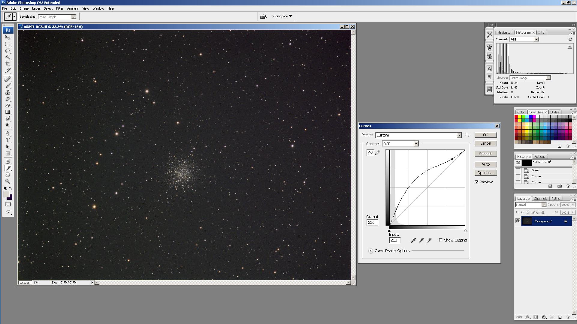
Figure 13. The fifth iteration in modifying the input/output relationship.
At some point in our iterative process, we will hopefully settle upon a version of the displayed image that we are pretty much satisfied with. This is the case with the image in Figure 14. Here, a final clipping of the low end of the pixel value distribution is performed to produce a nice dark background in the image. In comparing this image with the version in Figure 4, we can see that the majority of stars in this image are much more colorful and are not just white dots. The brightest stars in this image are not saturated (i.e, white cores surrounded by a thin halo of color, as in Figure 4). There are more smaller stars visible in the cluster and more variation in stellar magnitudes (the brighest stars in the cluster are not saturated), giving the cluster a more dimensional appearance.
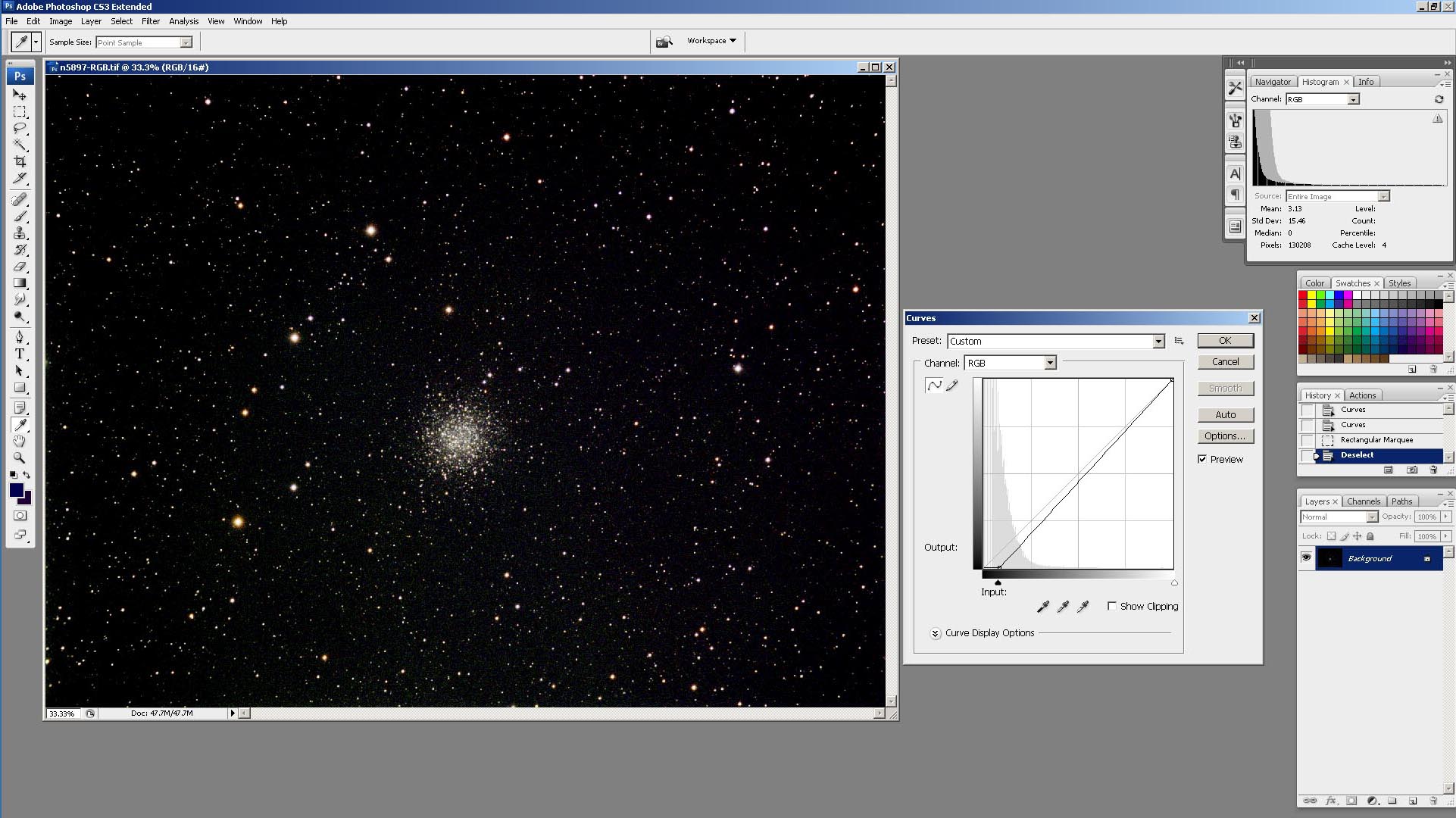
Figure 14. The final iteration in modifying the input/output relationship.
When you arrive at a version of the displayed image that you like, you can save it. Since you'll probably be using the image on a website or emailing it to friends, you'll most likely want to save it as a JPEG image. This will require that you convert the 16-bit TIFF version (which is what you've been working on in Photoshop) to an 8-bit version that can be saved as a JPEG. Don't worry about the loss of bits in the conversion— the saved JPEG will look just like the image displayed in Photoshop, because the displayed image is an 8-bit version of the TIFF image (remember that your computer monitor can only display 8-bit versions of images, regardless of how many bits the original image is). To convert the image into a form that can be saved as a JPEG, go to "Image" on the Photoshop Toolbar, select "Mode" from the drop-down menu, and check the "8 Bits/Channel" option in the list it provides (the "16 Bits/Channel" option will likely be checked since you've been working on a 16-bit TIFF file). Once that is done, go to "Save As..." under "File" on the Toolbar and save the image as a JPEG.
In summary, use of this iterative procedure can be effective in bringing out the details in the display of an imaged astronimcal object without producing excessive saturation of brighter elements (like stars or galaxy cores) in the image. It works particularly well on galaxies, where the challenge is to bring out the detail in the spiral structure of the outlying portions of the galaxy (where the brightness of the galaxy may be just above the backgound brightness) while preventing the bright central region from ending up just a white, featureless blob. It's also very effective on emission nebulas like M 42 that exhibit a wide range in brightness. So, how many iterations are needed to produce a good image? There's not a set number, but I've found that a greater number of smaller modifications to the input/output relationship in the "Curves" display are generally needed for objects with a greater range in brightness from the dimmest to the brightest image elements. Another thing that I've found is that, the more times you do this procedure, the better you get at it. There's no substitute for experience!
In comparing the images of the star field in Figure 14 and Figure 4, one thing that stands out is that, in Figure 4, the brighter stars have fairly sharp edges while, in Figure 14, the same stars look "softer" with more "fuzzy" edges. Bright stars in Figure 4 tend to have strongly saturated white cores surrounded by a thin halo of color that gives the stars an indication of their actual color. In contrast, bright stars in Figure 14 do not have strongly saturated cores but instead display their color more uniformly over the entire image of the star. The differences in the representation of (mostly brighter) stars in these two images are the result of how the image histograms were manipulated. "Soft" stars are a characteristic result of the type of contrast-stretching described in the previous section. Whenever you see "soft" stars in an astro-image in a publication or webpage, there's a good chance that the image was processed using this general type of contrast-stretching.
So, how does this type of contrast-stretching produce "soft" stars? Recall that the objective of this iterative contrast-stretching procedure is to increase the low pixel values in the image while holding the high pixel values at about the same. This will have the effect of decreasing the contrast between the brighest and dimmest pixels and allow more of the pixels to fit within the 0-255 range of displayed values. Suppose we take brightness measurements along a transect crossing a star in an image, as shown in Figure 15. The brightness curve for the transect in the original image is shown in Figure 16A. Since this is a relatively bright star, it has a large peak in brightness, making it much brighter than the other objects (like galaxies or nebulas) in the image that we might be interested in. Figure 16B shows the change in the brightness curve resulting from our contrast-stretching procedure. Note that the pixel values for the dimmer pixels have been increased (i.e., the base of the brightness curve has moved up), while the pixel values for the brightest pixels have remained the same (i.e., the peak in the brightness curve is the same). This has had the effect of decreasing the overall contrast (i.e., the difference) between the brightest and dimmest pixels.
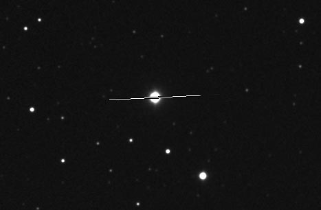
Figure 15. Transect across the image of a star.
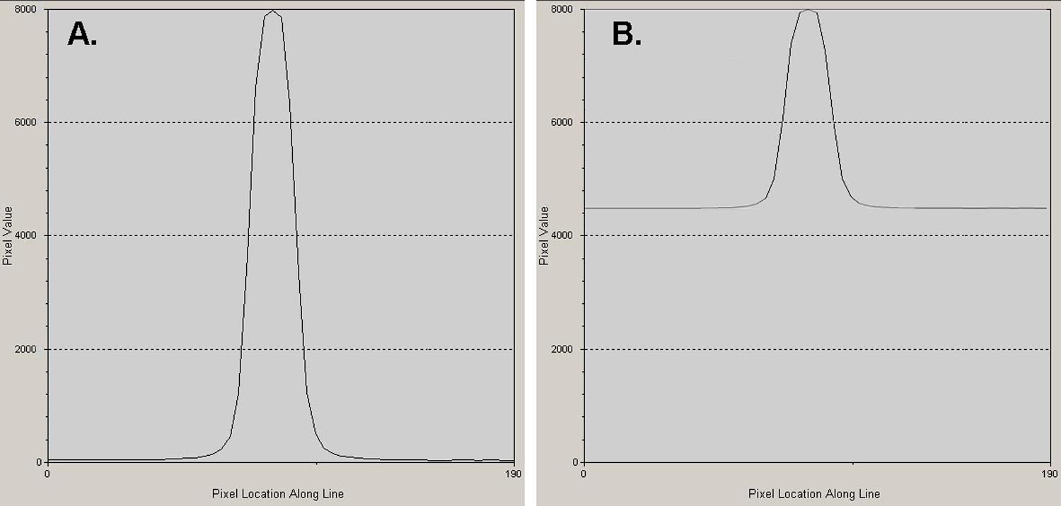
Figure 16. Brightness curves for the transect across the star in Figure 15: (A.) Original image; (B.) Stretched image.
As shown in Figure 17B, the objective of our contrast-stretching was to put the range of pixels values in the image mostly within the 0-255 range of brightness values that can be displayed on the computer monitor. When we try to apply this 0-255 brightness range to the curve in Figure 17A, we see that the range of pixel values won't completely fit in it. In the first section on this webpage, our solution to this problem was to clip the range of pixel values so that the object that we were interested in was in the 0-255 brightness range— this resulted in the image in Figure 4. But for the brighter stars in Figure 4, a large portion of their brightness curve is above the upper display limit (like in the example in Figure 17A). The image pixels corresponding to this part of the curve are saturated, and give rise to the white "core" of the brighter stars in Figure 4. In Figure 17A, the portion of the brightness curve for the star within the 0-255 range, but not within the saturated core, will not be saturated and will give the star its "halo" of color in the image, as with the brighter stars in Figure 4.
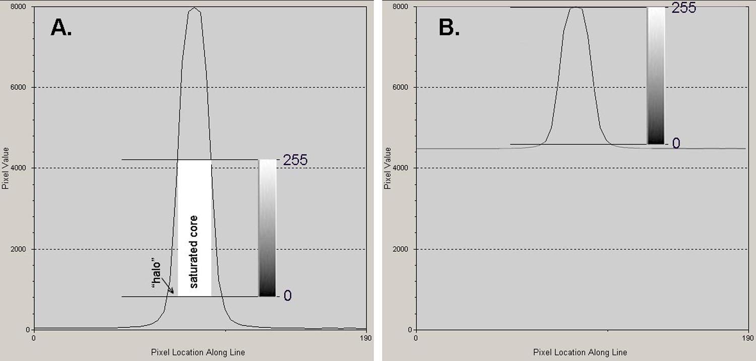
Figure 17. Brightness curves as in Figure 16, but also shown is the 0-255 range of display values (vertical bar with black-to-white gradient).
Since the brightness curve for the star in Figure 17B largely fits within the 0-255 display range, there is no saturated core and the star in the image would show a gradual change in brightness from its center to its edge. This is the case with the stars in Figure 14. In summary, "soft" unsaturated stars are a characteristic of images that have been contrast-stretched using the iterative procedure described in this webpage.
 Return to SOCO Image Processing Page
Return to SOCO Main Page
Return to SOCO Image Processing Page
Return to SOCO Main Page
Questions or comments? Email SOCO@cat-star.org