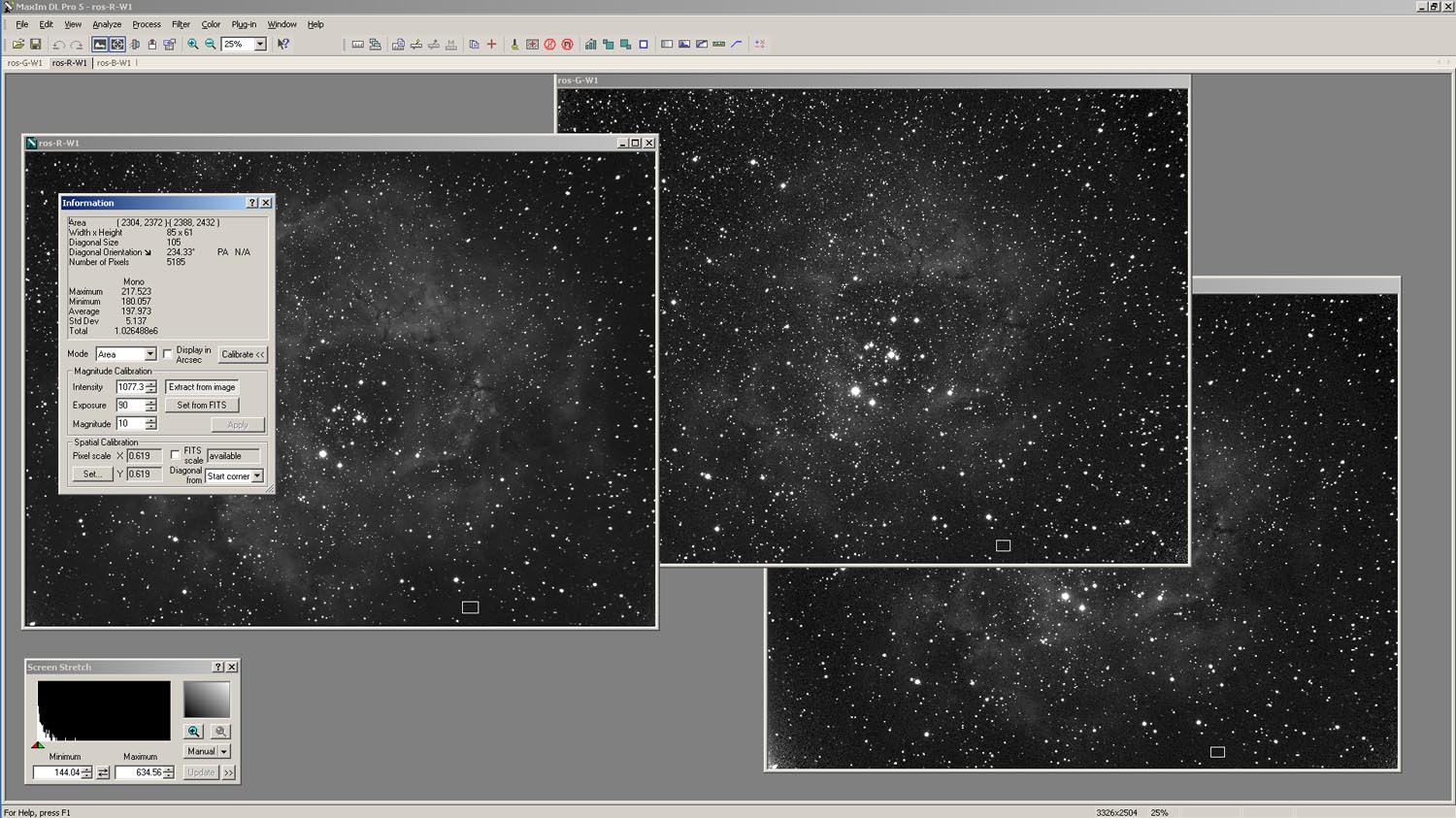
Figure 1. Using the Information Window in Maxim DL to determine average skylight values from selected areas (boxes) in images.
ADJUSTING IMAGERY FOR SKYLIGHT
(03 April 2015)
The clear night sky is dark, but not totally black. There are a number of sources that lead to a flux of light from the background night sky. If your observing location is near ground sources of light (illumination from buildings and vehicles, roadway lights, security lights, etc.), a portion of this light propagating upward into the atmosphere gets scattered back to the surface. In cities and densely populated urban areas, this leads to night skies that are not really dark and reveal only the brightest stars and planets. Away from cities, this is manefest as a dome of light projecting upward from the location of the city on the horizon. Even in sparsely populated areas, there is a component of background skylight. Some is light scattered downward from astronomical objects (particularly, the moon). Even in dark moonless night skies there is a faint downward flux of light in the form of airglow resulting from the interaction of energetic particles with the gases of the upper atmosphere. Background skylight is a problem in processing astronomical images not only due to its magnitude but also due to its ability to affect the color balance of the imagery. As long as the skylight component does not overwhelm the other features in the imagery, it is possible to adjust the imagery to remove its effects. Procedures for doing this are outlined on this page. Skylight is an additive feature in our astronomical imagery— its value in a given spectral band is added to the other photon fluxes in each pixel of the image. Numerically, this can be expressed as follows, Sg = Sobj,g + Ssky,g Equation 1b. Sb = Sobj,b + Ssky,b Equation 1c. Because skylight can affect the color balance of an image, adjustment for it should occur in the individual monochrome images for the red, green and blue spectral bands before they are combined into a color composite image. Measuring skylight involves identifying regions in the image that are essentially "empty space" away from the main object that we are imaging. This is usually not a problem, because most astro-imagers like to "frame" the object within the image so that there is some non-object border around it. A number of software tools can be used to measure the magnitude of the skylight component in imagery. Figure 1 shows three images of the Rosette Nebula opened in Maxim DL. These are the "master" red, green and blue monochrome images that will be combined to form a composite color image. The sets of images used to create these master images were aligned, stacked, corrected for optical artifacts (using flat frames), adjusted for zenith angle, processed to remove the hot pixels, thermal noise, and cosmic ray hits, and adjusted using weight factors based on G2V stars. They are pretty much ready for combining into the color composite, except that they have not been adjusted for the background skylight. To measure the magnitude of the skylight component in each image, the "Information Window" was opened from the "View" drop-down menu on the Maxim DL toolbar. This feature presents a variety of information about an opened image, including pixel statistics (average, standard deviation, etc.). If we select "Area" from the drop-down menu for the "Mode" feature, the application will allow us to draw (using the cursor) a box in an image. In this case, the pixel statistics reported by the Information Window will be for the portion of the image in the box. As shown in Figure 1, a small box has been drawn in the same location near the bottom of each of the three images. The location of this box was chosen to be outside the nebula and to not contain any obvious stars.
Sr = Sobj,r + Ssky,r Equation 1a.
in which S is the raw photon flux image data produced by the camera, Sobj is the photon flux from the object (outside the atmosphere) we are trying to image, Ssky is the photon flux from the sky background, and the r, g, and b subscripts refer to the red, green and blue spectral bands. As long as there are no noticeable gradients in skylight across the image (which should be reasonably true in narrow field-of-view imaging), then Ssky will be a constant over the area of the image. In this situation, adjustment is just a matter of quantifying the magnitude of Ssky and then subtracting this value (or a part of it, as we will see) from each pixel in the image.
Measuring Skylight
Figure 1. Using the Information Window in Maxim DL to determine average skylight values from selected areas (boxes) in images.
When each of the three images is made the "active" image, the pixel statistics for the box within it will be displayed in the Information Window. This allows you to collect skylight measurements for each image. The statistic you want is the average pixel value (in Figure 1, an average pixel value of 197.973 is listed for the currently "active" image). Write these values down. It's best to repeat this activity several times, with a new box drawn in the three images each time. Then you can average these values to get a better idea of the overall magnitude of skylight in each image. For example, suppose that we came up with average skylight values of 198, 209 and 137 for the red, green and blue images, respectively. This shows us that the magnitude of the skylight is greater in the red and green images than in the blue image. As we will see later, if we don't adjust for this, the color balance of our image will be messed up.
To correct the images based on our measurements, we could subtract 198 from each pixel in the red image, 209 from each pixel in the green image, and 137 from each pixel in the blue image. This would make the average background brightness in each image zero— corresponding to "black" in the display. However, it's generally not recommended that the images be adjusted in this way. This is because around half of the background pixels in an image will be greater than the average, and around half will be less than the average. When you subtract the average skylight value, the pixels that were less than the average will now have negative values. It's usually not good to have a lot of negative pixel values in an image.
A better approach is to normalize the skylight values according to the smallest average value. For our example, the average skylight value for the blue image (137) is the smallest. The difference between the average values for the green and blue images is 72, while the difference between the average values for the red and blue images is 61. So, we would subtract 61 from each pixel in the red image and 72 from each pixel in the green image. This results in the average background brightness being approximately equal among the three images, but not zero. For this example, the average background brightness would be around 137 and, since it's about the same in the red, green and blue images, it would correspond to a dark gray in the color composite. This non-zero average background brightness is sometimes called a "pedestal". It can be removed later through contrast-stretching of the color composite image.
The actual subtraction process is performed using "pixel math" tools that can be found in most image processing software packages. In Maxim DL, the "Pixel Math" tool can be found in the drop-down menu under "Process" in the toolbar. In AIP4WinV2, the "Pixel Math" tool can be found in the drop-down menu under "Enhance" in the toolbar.
The effects of adjusting the red, green and blue images for skylight on the resulting color composite image are shown in Figure 2. The left image was not adjusted for skylight. while the right image was adjusted by normailizing the skylight as described above. The un-adjusted image shows an yellow-green tint. If we display the average skylight values determined above as a color on the monitor, i.e., RGB = (198,209,137), we see that the resulting "color" is yellow-green (left side of Figure 3). Thus, it is the color of the skylight that corrupts the color balance of our color composite image. In contrast, normalizing the skylight values transforms the background color to a neutral gray (right side of Figure 3), which preserves the true color balance of the image.
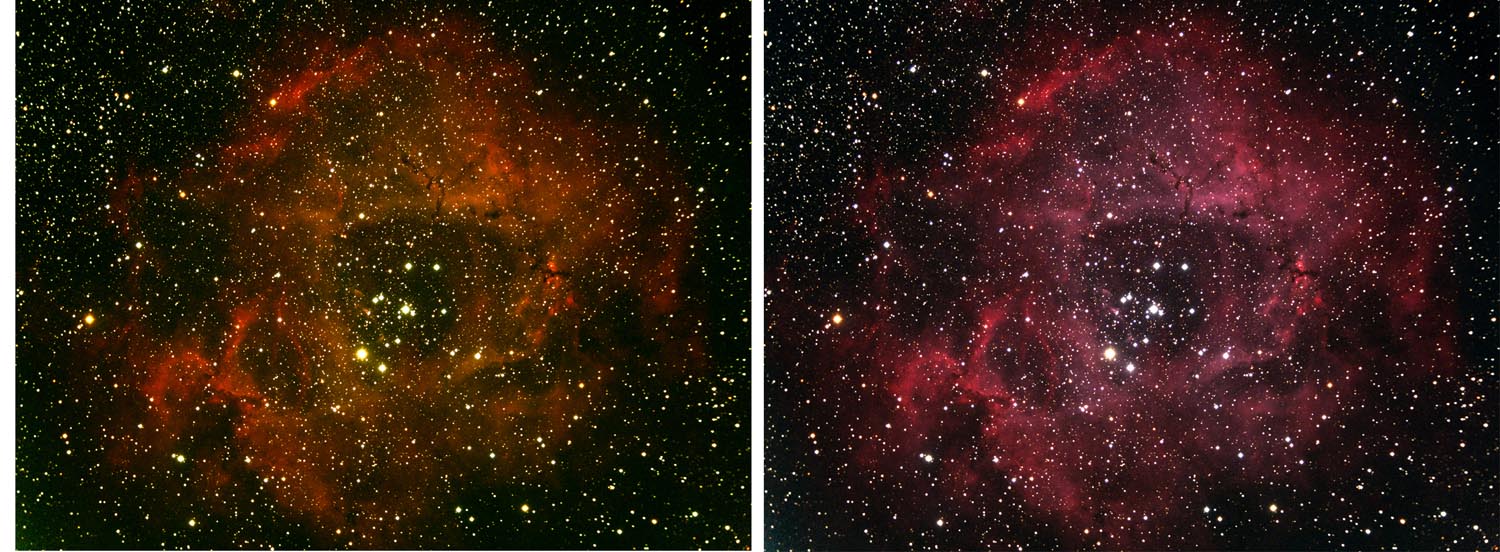
Figure 2. Effect of skylight brightness on color composite images; (left) no adjustment, (right) with normalization.
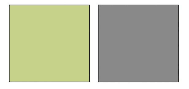
Figure 3. "Color" of the background skylight in the example color composite image; (left) no adjustment, (right) with normalization.
At this point you might wonder, why isn't the effects of skylight removed in applying the weight factors previously developed for image correction? The weight factors won't affect the background skylight because, in collecting the G2V star photon flux data used to evaluate the weight factors, the effects of the background were automatically subtracted out by the photometric procedure. That is why you can collect G2V star data for calculating the weight factors even on bright moonlit nights— the procedure will automatically remove the skylight effect. So, adjusting for skylight must be done in addition to applying the weight factors to the imagery.
In summary, adjusting for the background skylight is important in preserving the correct color balance in color composite images. Luckily, the procedure for doing this is easy and requires no additional information other than what can be derived from the imagery itself.
 Return to SOCO Image Processing Page
Return to SOCO Main Page
Return to SOCO Image Processing Page
Return to SOCO Main Page
Questions or comments? Email SOCO@cat-star.org