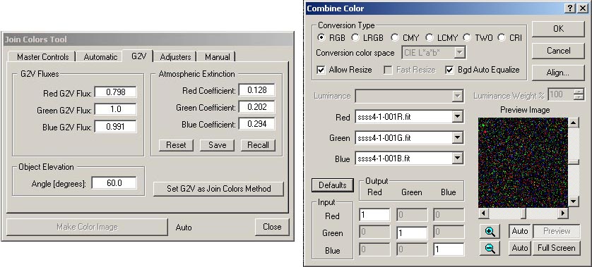
Figure 1. Join Colors tool (left) from AIP4WinV2 and Combine Color tool (right) from Maxim DL.
DETERMINING WEIGHT FACTORS
(29 March 2015)
(Revised 1 April 2015)
(Updated 4 July 2015)
To maintain the proper color balance within sets of red, green and blue images, the images must be corrected for differences in atmospheric transmissivity and effects related to the characteristics of certain imaging system hardware components (filters and camera sensor) before turning them into color composites. Figure 1 shows examples of software tools (from Maxim DL and AIP4WinV2) used to combine red, green and blue images into an RGB color composite. In the Join Colors tool, values for the atmospheric extinction coefficients for the red, green and blue bands must be specified. In addition, the elevation of the object images must be specified. With this information, the software will correct the imagery for elevation-related transmissivity effects by adjusting the image photon fluxes to the values the imagery would have if the imaged object were directly overhead. Also in the Join Colors Tool within the "G2V Fluxes" box are the values of the weight factors (the three boxes labelled "Red G2V Flux", "Green G2V Flux", and "Blue G2V Flux") that must be applied to the red, green and blue images. The Combine Color tool also has a place to enter the values of the weight factors— this is the three rows of boxes in the bottom left corner of the panel. The values of the weight factors are enterred in the diagonal row of boxes, one each for the red, green and blue spectral bands. In Figure 1, these boxes contain the default values— 1.
Figure 1. Join Colors tool (left) from AIP4WinV2 and Combine Color tool (right) from Maxim DL.
Mathematically, these corrections can be expressed as follows,
S'r = Sr / (Ar Wr) Equation 1a.in which the r, g, and b subscripts refer to the red, green and blue spectral bands. S is the raw photon flux image data produced by the camera, while S' is the corrected photon flux data. A is the atmospheric transmittance and W is the hardware-related weight factor. A is a function of the zenith angle (SZA) of the object,
S'g = Sg / (Ag Wg) Equation 1b.
S'b = Sb / (Ab Wb) Equation 1c.
Ar = 10 -0.4 kr [sec(SZA)-1] Equation 2a.where k is the atmospheric extinction coeffient. The zenith angle is the complement of the elevation angle.
Ag = 10 -0.4 kg [sec(SZA)-1] Equation 2b.
Ab = 10 -0.4 kb [sec(SZA)-1] Equation 2c.
The values of these weight factors are based on one very important assumption, namely, that the relative photon fluxes of a G2V star are identical to white light. Numerically, this means that, for Equations 1a, 1b and 1c, S'r = S'g = S'b. Our sun is a G2V star and, by definition, the light coming from it is "white light". This is why, in regular photography, we expose our digital camera to sunlight falling on a white (or gray) card to set the "white balance" of the camera. The procedure outlined above is designed to do the same thing— to provide a "white card" for calibrating our astro-images to have the right color balance. When applied to our images, the weights calculated using this procedure will make G2V stars appear white, assuming that our display monitor is properly color-calibrated and the stars are not saturated in the image (saturated stars always appear white because their red, green and blue values in the image are at the maximum). If the G2V stars in the image have the right color balance, then presumably all the other objects in the image also have the right color balance. More details on using G2V stars for calibrating astro-images can be found in "The Handbook of Astronomical Image Processing" by Richard Berry and James Burnell (Willmann-Bell Publishers, Richmond, VA, 2009).
In the AIP4WinV2 Join Colors tool, you could use default values for the extinction coefficients. However, on another page, I've demonstrated that it's easy to determine your own k values for your location. The bonus in doing this is that the same data set that you collected for determining atmospheric extinction coefficients can be used to determine the values of the weight factors. The catch is that you have to determine the extinction coefficients first, because they're used in the evaluation of the weight factors. Physically, the weight factors are in part determined by the quantum efficiency of the camera sensor (CCD or CMOS chip) and the transmissivities of the filters. An example of the quantum efficiency of an imaging sensor is shown in Figure 2.
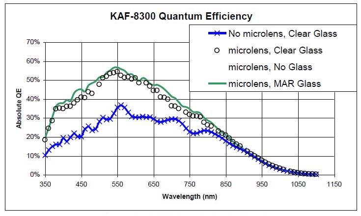
Figure 2. Quantum efficiency (QE) as a function of wavelength for the KAF-8300 sensor in the QSI Model 583 camera.
Source: Device Performance Specification, KODAK KAF-8300 IMAGE SENSOR, Revision 5.4 MTD/PS-0996, 13 Sept. 2010, KODAK, Inc.
As indicated in Figure 2, the response of an imaging sensor varies as a function of wavelength. So, the ability of the sensor to capture light is different for different spectral bands. The KAF-8300 is more effective in capturing photons of green light than photons of red or blue light. This relative effectiveness affects the color balance among sets of red, green and blue images acquired by the camera. Every type of imaging sensor is different in this respect, so weight factors derived for your make and model of camera will most likely be different from those determined for another make and model of camera.
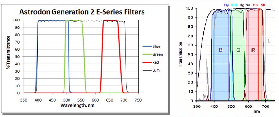
Figure 3 shows transmissivity curves for a set of commercially available red, green and blue filters. While most commercially available astronomical filters have peak transmissivities near 100%, the exact spectral range for each band (red, green and blue) can vary between manufacturers and models. These differences in spectral sensitivity can affect the color balance among sets of red, green and blue images acquired through the filters. Again, every filter set is different in this respect, so weight factors derived for the filter set you use will most likely be different from those determined for filters from another provider.
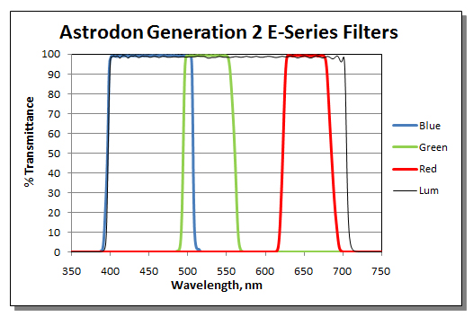
Figure 3. Transmissivities (%) for a set of Astrodon Generation 2 E-Series filters.
Source: Astrodon Astronomy Filters.
The weight factors incorporate the effects of other features besides the quantum efficiency of the camera sensor and the transmissivities of the filters, such as the basic transmissivity of the atmosphere in the zenith direction (SZA = 0). The atmospheric transmissivities calculated using Equations 2a, 2b and 2c are relative to the atmospheric transmissivity in the zenith direction. For the zenith direction, Equations 2a, 2b and 2c yield Ar = Ag = Ab = 1. So, Equations 2a, 2b and 2c are only used to normalize the effects of atmospheric transmissivity for images acquired with different zenith angles. In practice, the weight factors implicitly absorb the effects of all the other factors that aren't explicitly determined in processing the imagery.
All this means is that the weight factors for your astro-imaging setup will most likely be unique and typical values will have to be determined from the analysis of imaging data. Luckily, determining weight factors is easy and, if you've previously collected imaging data to evaluate atmospheric extinction coefficients, you've already got the data to do it. If you haven't done this, go ahead and collect the data and do it because, as I previously said, you need to know the values of the extinction coefficients in order to calculate the weight factors. The remainder of this discussion will describe the procedure for evaluating weight factors.
To illustrate the procedure for calculating weight factors, we'll use data originally acquired for G2V stars to determine atmospheric extinction coefficients. Two basic types of data were obtained in the process of determining extinction coefficients: (1.) raw (uncorrected) photon fluxes (S) in the red, green and blue spectral bands measured for G2V stars using the Color Calculator tool in AIP4WinV2, and (2.) corresponding values of stellar elevation angle (SEA) for the G2V stars determined from the acquisition times of the images. Figure 4 shows a portion of a spreadsheet with these data for one of the G2V stars. Values of Sr, Sg, and Sb are in columns B, C, and D, respectively, while corresponding values of SEA (in degrees) are in column F. The data within a column are arranged in four groups because these groups correspond to the four episodes of image acquisition during the observing session. As the data indicate, the star started out fairly high in the sky (SEA around 50 degrees above the horizon) when the first set of images was acquired, and ended up very close to the horizon (SEA around 7 degrees above the horizon) during the acquisition of the last set of images. The photon flux data behaves as we would expect, with values generally decreasing as the elevation angle decreased due to increasing absorption and scattering of the light.
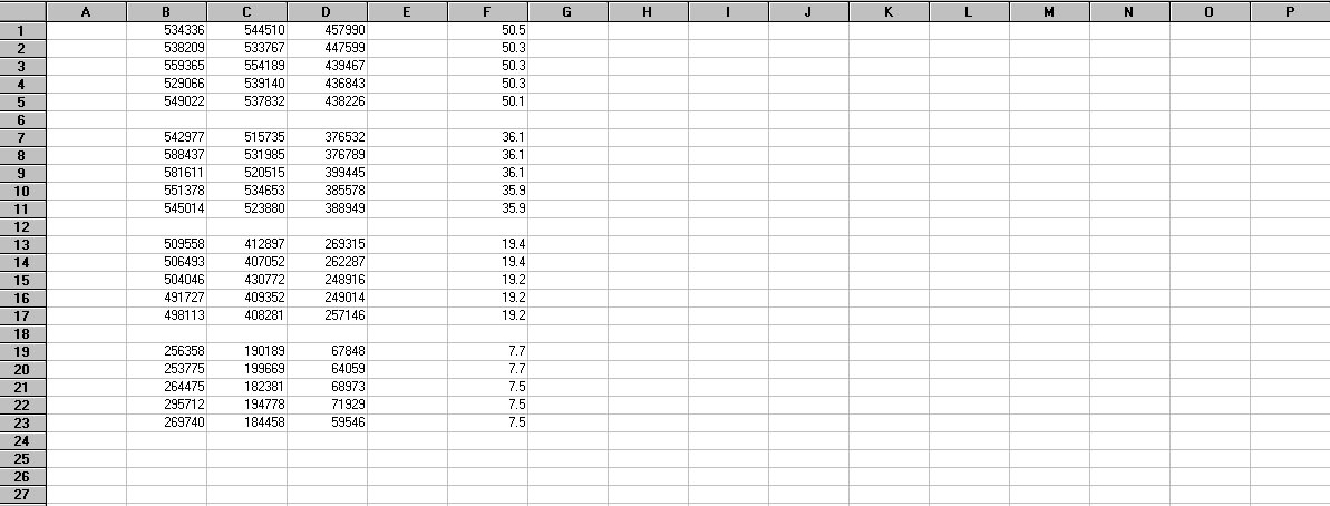
Figure 4. Portion of a spreadsheet showing photon flux data (Columns B-D) and elevation angles (column F) for the G2V star HD26749.
The first calculation to be made is computing the stellar zenith angle (SZA). SZA is the complement of SEA, so SZA = 90 - SEA (in degrees). Computed values of SZA for our example are presented in column G of the spreadsheet (Figure 5).

Figure 5. Spreadsheet from Figure 4 showing the computed values of SZA in Column G.
The values of SZA are used to compute the values of atmospheric transmissivity A using Equations 2a, 2b and 2c. In Figure 6, values of Ar are shown in column I, Ag in column J, and Ab in column K. As stated earlier, you must have values for the atmospheric extinction coefficients k in order to solve for A. From previous analysis, we know that kr = 0.1380, kg = 0.2050, and kb = 0.3313 for this data set. Note in the spreadsheet that the values of A decrease as the star gets closer to the horizon. This is what we would expect as the light from the star has to pass along a longer optical path through the atmosphere as it gets closer to the horizon.
I provide a computer application for calculating atmospheric transmissivity from the elevation angle of the star and the appropriate value of the extinction coefficient.
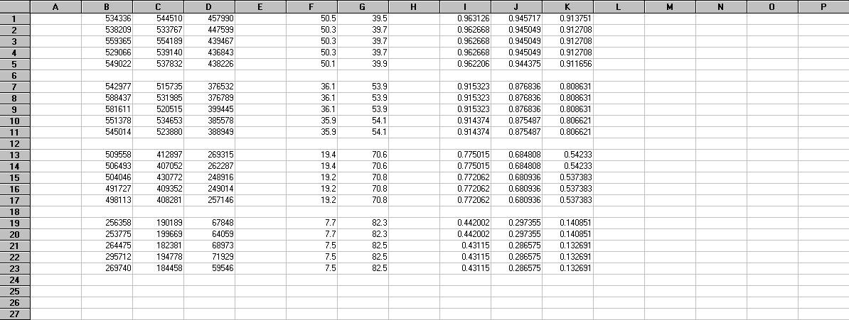
Figure 6. Spreadsheet from Figure 5 showing the computed values of A in Columns I-J.
We're almost finished with the calculations. If we divide each value of S (columns B, C and D) in the spreadsheet by its corresponding value of A (columns I, J and K), we correct the photon fluxes for the changes in atmospheric transmissivity associated with stellar elevation angle. These corrected values are presented in columns M, N and O of Figure 7. These corrected fluxes represent the fluxes that would be measured if the target star was always directly overhead (i.e., SEA = 90 degrees). Looking down the the corrected values in a column, you can see that they have roughly similar magnitudes (accounting for random observation-to-observation variations). This shows that our previously determined k values were good.
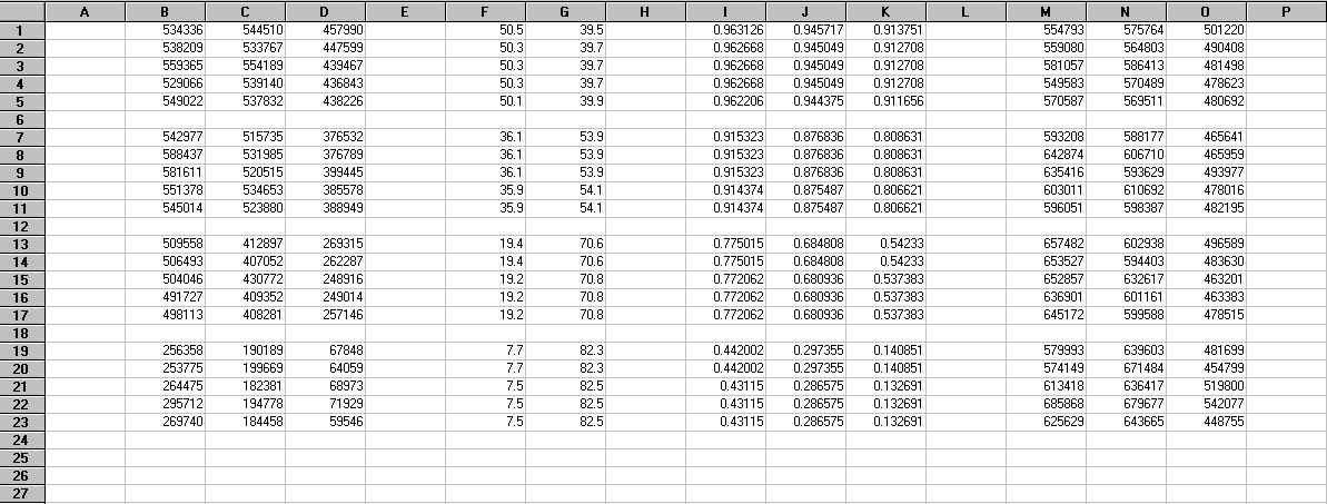
Figure 7. Spreadsheet from Figure 6 showing the computed values of S/A in Columns M-O.
Now, we calculate the averages of the S/A values in each column. These values are shown in Figure 8 next to the red arrow. So, the average value of S/A for the red spectral band was 610533; the average value of S/A for the green spectral band was 608306; and the average value of S/A for the blue spectral band was 482534. We will normalize these three averages by the largest of the three, in this case, 610533. The result is shown in Figure 9.
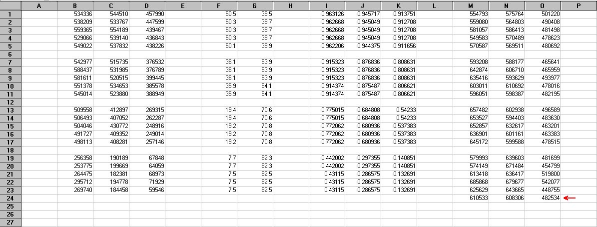
Figure 8. Spreadsheet from Figure 7 showing the average values of S/A (indicated by the red arrow) for the data in columns M-O.
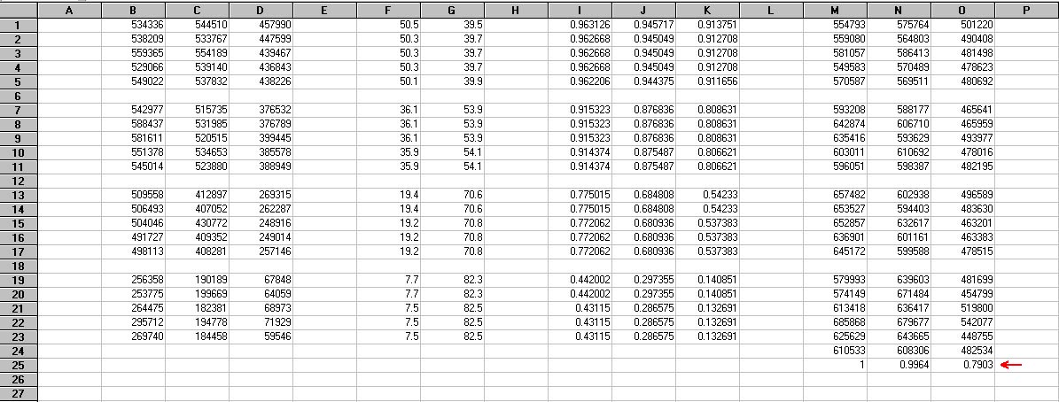
Figure 9. Spreadsheet from Figure 8 showing the normalized average values of S/A (indicated by the red arrow) for the data in columns M-O.
These three normalized values represent the weight factors that we are looking for. So, Wr = 1, Wg = 0.9964, and Wb = 0.7903 for the data from this star (note that one weight will always be 1 and the other two will be less than 1). This normalization satisfies the assumption that we made about G2V stars— that the photon fluxes in the red, green and blue spectral bands are equal. So, when these factors are applied to our atmospherically corrected images, they will force the photon fluxes in the three spectral bands to be equal. Thus, G2V stars will appear white, and presumably all other features in the imagery will also have the proper color balance.
If we analyze the data for other G2V stars, the values for the three weight factors should be roughly the same. To correct our raw imagery, the raw photon flux value acquired for each image pixel is divided by the calculated values of the weight factors (and atmospheric transmissivities) as indicated in Equations 1a, 1b and 1c. This is what software tools like those shown in Figure 1 do when you use these weight factors in them.
Table 1 shows values determined for the atmospheric extinction coefficients and weight factors from recent observing sessions at SOCO. The value for each date was derived from the data from four G2V stars. All observations were made on nights following cold front passages— skies were clear, temperatures were cold, and humidities were very dry. SOCO is around 1 km above sea level.
Table 1. Examples of values for extinction coefficients and weight factors.
|
In "The Handbook of Astronomical Image Processing" (Willmann-Bell Publishers, Richmond, VA, 2009), Richard Berry and James Burnell suggest the following values: Wr = 1, Wg = 0.93, and Wb = 0.78. These are fairly close to the average values in Table 1, although the value suggested for the green spectral band is somewhat lower than that in Table 1. Since all imaging setups are different, it's best to just calculate your own values.
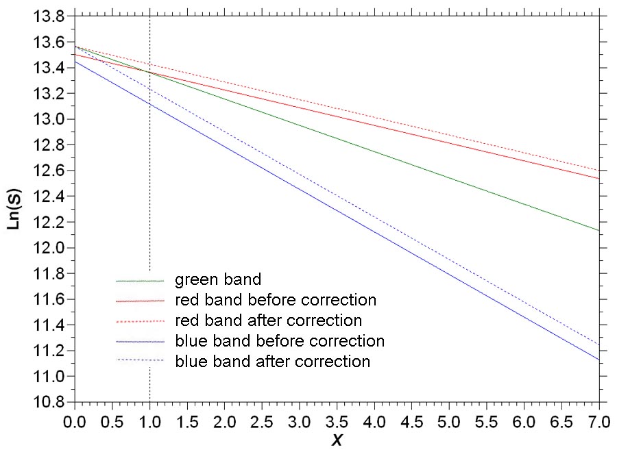
As previously stated, the values used for the weight factors in producing a color composite image can affect the color balance in the resulting image. In fact, we choose the weight factor values to intentionally produce a desired color balance— hopefully one that results in a rendition of the imaged object in a manner that approximates it's "true color". Figure 10 shows a graph of the natural logarithm of the stellar photon flux (S) for the red, green and blue spectral bands versus the optical air mass (X) for the G2V star used in the example on this page. The slopes of the lines on this graph represent the values of the atmospheric extinction coefficients (k). The solid lines in the graph represent the relationships before correction. As indicated in the graph, the relationships for the red and green spectral bands pretty much satisfy the assumption that the photon fluxes of G2V stars are equal in these spectral bands. For this reason, the values of Wr and Wg in Table 1 are both equal to 1 (at least approximately), indicating that little color balance correction is needed for these two spectral bands.

Figure 10. Graph of Ln(S) for the red, green and blue spectral bands versus X for a G2V star.
This is not the case for the blue spectral band. The intercept of the solid blue line with the y-axis at X = 1 (SZA = 0 degrees) in Figure 1 is substantially below the corresponding intercepts of the lines representing the relationships for the red and green spectral bands. As indicated in Table 1, the average stellar photon flux in the blue spectral band is only around 80% of the fluxes in the other two spectral bands. Thus, to bring about G2V correction, the values of S in the image for the blue spectral band are divided by Wb. This boosts the blue component in the color composite. In Figure 10, this correction is represented by the dotted blue line in the graph, which now intercepts the y-axis at approximately the same point as the solid red and green lines.
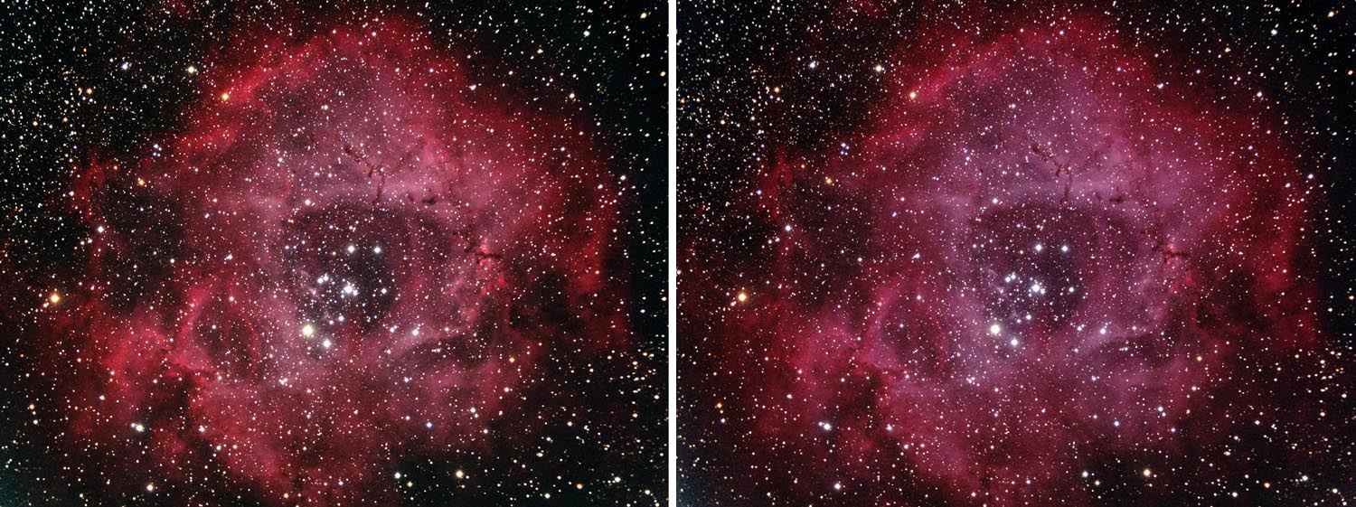
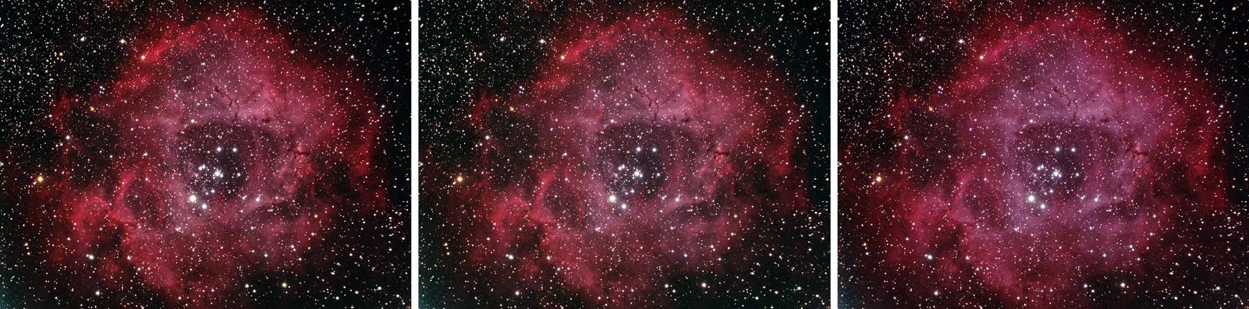
Figure 11. Color composite images of the Rosette Nebula. (left) Wr = Wg = Wb = 1; (right) Wr = 1, Wg = 0.9853, and Wb = 0.8154.
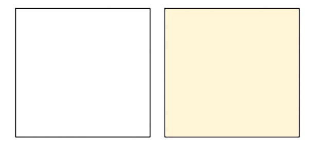
The result of this correction on image color balance can be visualized in Figure 11. The left image in the figure was produced without correction (Wr = Wg = Wb = 1), which corresponds to the solid red, green and blue lines in Figure 10. The right image in the figure includes the G2V correction for the blue spectral band (corresponding to the dotted blue line in Figure 10) and a small correction for the green band according to the average weight factors in Table 1. As a result, the overall rendition of the nebula is slightly bluer (or maybe "pinker") in the right image in the figure. According to our assumptions involving the equality of the photon fluxes for G2V stars, any (unsaturated) G2V stars in the right image in the figure should appear white, with the remainder of the features in the image rendered according to this color balance. As indicated in Figure 10, the basic assumption of the correction procedure described above is that the stellar photon fluxes in the red, green and blue spectral bands are equal for G2V stars viewed at the zenith (SZA = 0) through 1 air mass (X = 1). This results in G2V stars being rendered as white in the processed color composite images. I have a problem with this— although we are looking directly upward along the shortest optical path through the atmosphere, the light from the astronomical target still has to pass through 1 air mass to reach us. While the effects of atmospheric transmissivity in this situation should be at a minimum compared to when stellar zenith angles are greater than zero, there still should be substantial scattering and absorption of light at X = 1. This should be particularly true for blue light, since the clear atmosphere is very good at scattering blue light (that is why "the sky is blue"). This could explain why the line in Figure 10 representing the uncorrected relationship between Ln(S) and X for the blue spectral band (the solid blue line) falls substantially below the corresponding lines for the red and green spectral bands at X = 1. My feeling is, if the stellar photon fluxes in the red, green and blue spectral bands for G2V stars are equal, this should occur outside the atmosphere, before the atmosphere has a chance to scatter and absorb the light. These exoatmospheric conditions correspond to zero air mass (i.e., X = 0). The relationships shown in Figure 10 can be extrapolated to X = 0, as shown in Figure 12. When we do this, two things become apparent— (1.) the three lines representing the red, green and blue photon fluxes do roughly converge; and (2.) at X = 0, the photon flux in the green spectral band is the greatest (the flux for the red spectral band was the greatest at X = 1). The rough converegence of the three lines does suggest that the assumption of the equality of the three fluxes is not unreasonable. The blackbody emittance of G2V stars should peak in the green wavelengths, which could explain why the observed flux in the green spectral band is the greatest at X = 0. The lack of complete converegence at this point could be related to characteristics of the imaging system (quantum efficiency of the camera sensor and transmissivities of the filters), as suggested earlier on this page. Figure 12. Graph of Ln(S) for the red, green and blue spectral bands versus X as in Figure 10 extrapolated to exoatmospheric conditions. To perform an exoatmospheric G2V correction on the relationships shown in Figure 12, we need to evaluate a set of weight factors that make the photon fluxes in the red, green and blue spectral bands equal at X = 0. If W1,r, W1,g and W1,b are the weight factors used to equalize the red, green and blue photon fluxes at X = 1 (i.e., the values in Table 1), and W0,r, W0,g and W0,b are the weight factors needed to equalize the red, green and blue photon fluxes at X = 0, then W0,g = 1 Equation 3b. W0,b = (W1,b/W1,g)(ekb/ekg) Equation 3c. Table 2. Summary of weight factors determined for the two types of G2V correction. The result of this correction on image color balance is shown in Figure 13. As in Figure 11, the left image was produced without correction (Wr = Wg = Wb = 1). The right image in Figure 13 shows the previous result of G2V correction made at X = 1 (Wr = 1, Wg = 0.9853, and Wb = 0.8154). The center image in Figure 13 shows the result of G2V correction made at X = 0 (Wr = 0.9672, Wg = 1, and Wb = 0.9206). Figure 13. Color composite images of the Rosette Nebula. (left) Wr = Wg = Wb = 1; (center) Wr = 0.9672, Wg = 1, and Wb = 0.9206; (right) Wr = 1, Wg = 0.9853, and Wb = 0.8154. Comparing the results in Figure 13, it is apparent that the image involving G2V correction at X = 0 ("exoatmospheric correction") does not have as much of a blue tint as the image involving G2V correction at X = 1. It's color balance is intermediate between the other two versions, but closer to that of the uncorrected version. Average photon flux values in the red and blue spectral bands were determined for portions of the images with bright nebula. The ratios of the red to blue photon fluxes were around 1.305 for the uncorrected image, 1.271 for G2V correction at X = 0 (exoatmospheric correction), and 1.209 for G2V correction at X = 1. Thus, the uncorrected image is "redder" than the image with exoatmospheric correction, and the image with G2V correction at X = 1 is "bluer" than the image with exoatmospheric correction. One consequence of exoatmospheric G2V correction is that G2V stars will not appear white in the corrected composite color images. This is because the corrected relationships for the red, green and blue spectral bands do not intersect at X = 1 in Figure 12 as they did in Figure 10. If we convert the set of values of Sr, Sg and Sb at X = 1 from Figure 12 to a relative scale ranging from 0 to 255, where 255 represents the largest value (Sr), and express this as an RGB value on a display monitor, we get RGB = (255,246,215). The resulting "color" is shown on the right side in Figure 14 along with the white color of G2V stars in images with G2V correction at X = 1. Thus, this analysis shows that G2V stars in color composite images produced using exoatmospheric G2V correction should appear slightly "yellower" than corresponding stars in images with G2V correction made at X = 1. Maybe this is why some people say that the sun is a "yellow star". Figure 14. Relative unsaturated colors of G2V stars, (left) G2V correction at X = 1, (right) G2V correction at X = 0. My current opinion is that exoatmospheric G2V correction provides the best objective approximation to the "true color" of imaged astronomical objects in color composites constructed from imagery acquired in the red, green and blue spectral bands. Values of weight factors needed to perform this correction can be calculated using Equations 3a, 3b and 3c from values like those in Table 1 determined using the analytical procedures described on this page. As stated above, one of the things that determines the values of the weight factors is the spectral characteristics of the filters used in the imaging system. While most astronomical filters used in imaging cover the same basic spectral bands (i.e., red, green and blue), the specific wavelengths of light that a filter allows to pass may be somewhat different among different manufacturers. For example, Figure 15 shows the spectral bandpass characteristics of red, green and blue filters provided by two popular filter manufacturers— Astrodon and Baader. Figure 15. Spectral bandpass characteristics of red, green and blue filters from two manufacturers, (left) Astrodon, (right) Baader. The values determined as appropriate for Exoatmospheric G2V Correction using these two types of filters are presented in Table 3. The values for Baader are those taken from Table 2. For Astrodon, the weight values were determined using the procedures described above from photometric data obtained for seven G2V stars observed on 29 June 2014 (I switched from Astrodon to Baader filters at the start of 2015). As shown in the table, there are significant differences in the weight factor values between the two types of filters. For the Baader filters, the values of the weight factors for all three spectral bands are relatively large— greater than 0.9. For the Astrodon filters, however, the weight factor for the red band is considerably smaller than the values for the other two spectral bands. This is likely related to the fact that the range of bandpass wavelengths for the Astrodon red filter is considerably narrower than the corresponding range of bandpass wavelengths for the Baader red filter (see Figure 15). Since the transmissivities for the two types of filters are about the same, the narrower range of bandpass wavelengths for the red Astrodon filter allows less light to reach the camera as compared to the red Baader filter. To maintain the proper balance among the three spectral bands (as determined by the analysis involving G2V stars), the value of Wr for the Astrodon filter is proportionately smaller— thus, when this weight factor is applied to the pixel values in the red images (Equation 1a), their pixel values will be appropriately increased. Regardless of the spectral characteristics of a set of filters, the analysis described on this webpage will produce a set of weight factors that will insure the proper color balance in your imagery. Table 3. Weight factors for Exoatmospheric G2V Correction for filters from two manufacturers. These results aren't meant to suggest that one manufacturer's filters are "better" than another's. What they emphasize is the importance of determining the values of the weight factors for your imaging system, once you've chosen a set of filters. Questions or comments? Email SOCO@cat-star.org
An Alternate Approach— Exoatmospheric G2V Correction
W0,r = (W1,r/W1,g)(ekr/ekg) Equation 3a.
in which e is the base of natural logarithms. Using the weight factor and extinction coefficient values from Table 1 in Equations 3a, 3b and 3c, we get W0,r = 0.9672, W0,g = 1, and W0,b = 0.9206. The corrected relationships are represented by the dotted red and blue lines in Figure 12. Overall, the G2V corrections made at X = 0 are smaller than the G2V correction made at X = 1. The differences in the two sets of weight factors are summarized in Table 2.
Effects of Filters on Weight Factors
Sources: Astrodon Astronomy Filters
Baader News 05/2008: "Baader announces Anti-reflective LRGBC filter-line to complement
Baader Narrowband CCD-Emission Line-filters"
 Return to SOCO Image Processing Page
Return to SOCO Main Page
Return to SOCO Image Processing Page
Return to SOCO Main Page