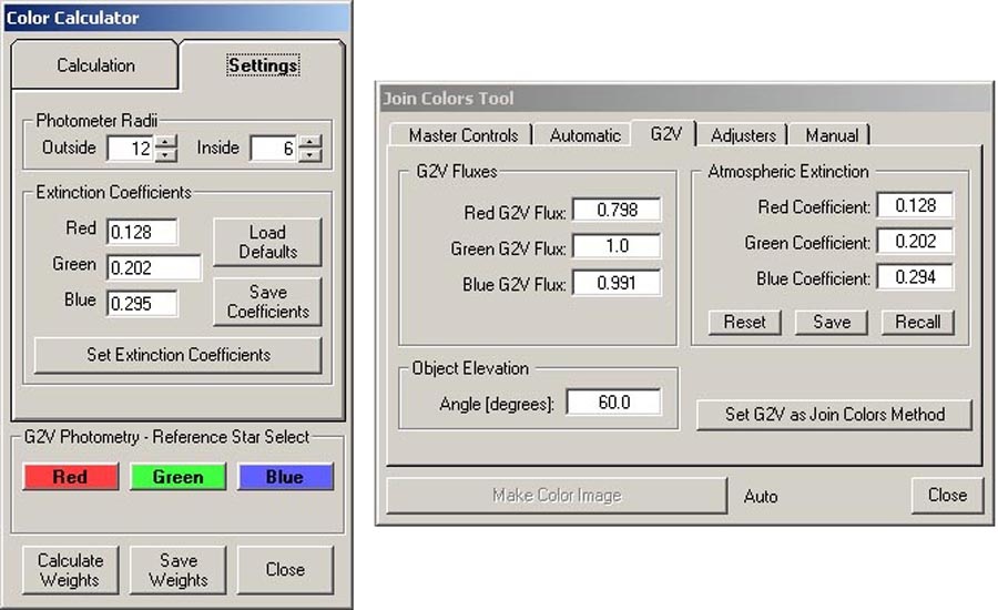
Figure 1. Color Calculator (left) and Join Colors Tool (right) functions in AIP4WinV2.
DETERMINING ATMOSPHERIC EXTINCTION COEFFICIENTS
(March 2015)
(January 2016)
While the night sky may appear "clear", the atmosphere through which we make our astronomical observations has a profound effect on the light passing through it. As light from an exoatmospheric object passes through the atmosphere, it can be absorbed and/or scattered by the gaseous contituents of the atmosphere and the aerosol particles suspended in the atmosphere. The longer the optical path through the atmosphere between the object and the observer, the more the light gets absorbed and scattered. Thus, objects closer to the horizon are affected more than those higher in the sky. In addition, the degree to which the light is affected depends on its wavelength. Numerically, these effects are quantified by factors called "extinction coefficients" (k) which are used to calculate the transmittance of the atmosphere to light. In astro-imaging, extinction coefficients become important because the elevation of the imaged target above the horizon may change appreciably during the acquisition of a sequence of images. Thus, the atmospheric transmittiance when the object was high in the sky would not be the same as the atmospheric transmittiance when the object was low in the sky. It wouldn't be as much of a problem if all wavelengths of light were affected equally, but that's not the case. Blue light is affected more than green light, and green light is affected more than red light. Thus, images acquired when the object was at different elevations not only have differences in overall magnitude, but also differences in color balance. These differences must be corrected for when combining sequences of RGB images to produce "true color" composites. A number of image processing functions make use of atmospheric extinction coefficients. Two examples are shown in Figure 1. In the Color Calculator in AIP4WinV2, the values of the extinction coefficients in the red, green and blue wavebands must be specified in order to calculate the photon flux weight factors from G2V star images. These weights are necessary to achieve proper color balance when making color composite images, and so they also appear in the AIP4WinV2 Join Colors Tool. Similar functions can be found in other image processing packages. In these functions, the extinction coefficients are used to correct red, green and blue images to how they would appear if the imaged target were directly overhead (zenith angle = 0). This normalizes all the images and removes the effects of differences in target elevation. This correction must be done before applying the weight factors to the images.
Figure 1. Color Calculator (left) and Join Colors Tool (right) functions in AIP4WinV2.
As indicated in Figure 1, image processing packages often provide default values for the atmospheric extinction coefficients. These default values are often based on general atmospheric transmissivity conditions for certain observing sites, such as "low-altitude, humid" or "high-altitude, dry" sites. However, k values can vary considerably from site to site, and even at a given site from season to season. As it turns out, extinction coefficients are easy to determine, so it is possible to come up with your own values that are appropriate for your site. The remainder of this page outlines a procedure for determining the values of atmospheric extinction coefficients.
In this procedure, you'll be imaging G2V ("sun-like") stars, which are stars in the same spectral class as our sun. Actually, you could image stars in practically any spectral class to determine k values, but using G2V stars also allows you to determine the weight factors once you've evaluated the extinction coefficients. You'll select a group (4 is good) G2V stars such that they are near the horizon at the start of your imaging session and are high in the sky when they culminate (reach their highest point). It's not necessary for the stars to pass directly overhead— a maximum elevation of 50 to 60 degrees above the horizon is okay. A typical imaging session to collect data for determining extinction coefficients will last 3 to 4 hours.
There are a number of sources for finding lists of G2V stars. My favorite is the list provided by Dr. Dale E. Gary, Distinguished Professor of Physics at the New Jersey Science & Technology University (NJIT). It includes several hundred stars drawn from the Hipparcos Catalog.
To plan your imaging session, choose a group of G2V stars that will have just risen above the horizon once it gets good and dark. You'll want to get your first set of images of these stars when they have an elevation above the horizon of not more than 20 degrees. Over the next few hours, you'll periodically acquire additional sets of images of these stars as they rise. Your last set of images will be acquired when the stars are near culmination. The alternate procedure is to start when the stars are near culmination and follow them down the sky, acquiring your last set of images just before the stars set. A good planetarium software application, like Cartes du Ciel or Starry Night, can be useful in planning your imaging session.
To explain the procedure, I'll use an example in which I imaged four G2V stars over several hours as they moved down the sky from near culmination to just before setting. The imaging session started at 9:11 PM CDT on 11 March 2015 and ended at 12:49 AM CDT on 12 March 2015. Characteristics of the 4 stars are summarized in Table 1.
Table 1. Characteristics of the four G2V stars used in the example.
|
Figure 2 shows the elevation and azimuth positions of the four stars when imagery was acquired. Stars #3 and #4 were separated by approximately 1 degree, so their plotted positions overlap in the figure. Each black dot represents a set of 5 separate images acquired in rapid succession for each star. Multiple images make statistical analysis of the data more robust. I had intended to acquire 4 sets of images for each star. Unfortunately, stars #3 and #4 had sunk behind a treetop at the time of the fourth acquisition, so only 3 sets of images were acquired for these two stars.
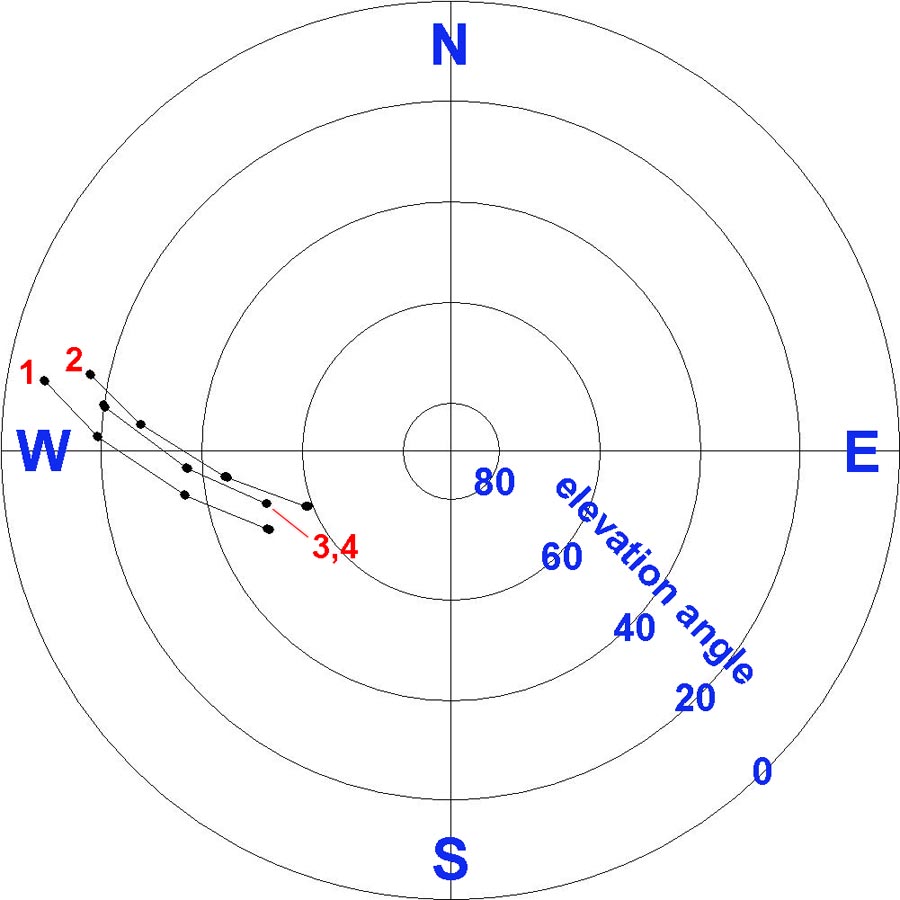
Figure 2. Elevation and azimuth positions of the four stars when imagery was acquired (black dots). Red numbers are the star numbers in Table 1.
Images were acquired using a QSI Model 583 monochrome digital camera. Images were acquired through Baader red, green and blue filters. An example is shown in Figure 3. In acquiring images for determining atmospheric extinction coefficients, it is important that the image of the target star not reach saturation. This requires proper setting of exposure times for each star, and the same exposure time must be used for all images of a given star during the entire imaging session. My QSI camera is controlled using Maxim DL, so I can use the Information Window in the Expose Tab of the Camera Control panel to display the maximum pixel value for the target star isolated within a small rectangular subframe of an image (see Figure 4). In this way, I can choose an exposure time that will prevent saturation of the target star image. For the 6th-magnitude stars in Table 1 (stars #1 and #2), an exposure of 4 seconds was used. For the 7th-magnitude stars in Table 1 (stars #3 and #4), an exposure of 5 seconds was used. For this example, a total of 210 monochrome images (70 RGB triads) were acquired over the course of the imaging session.
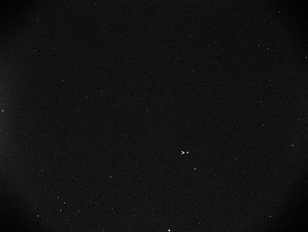
Figure 3. Example of a monochrome image of HD26749 (star #1), indicated by the ">" pointer.
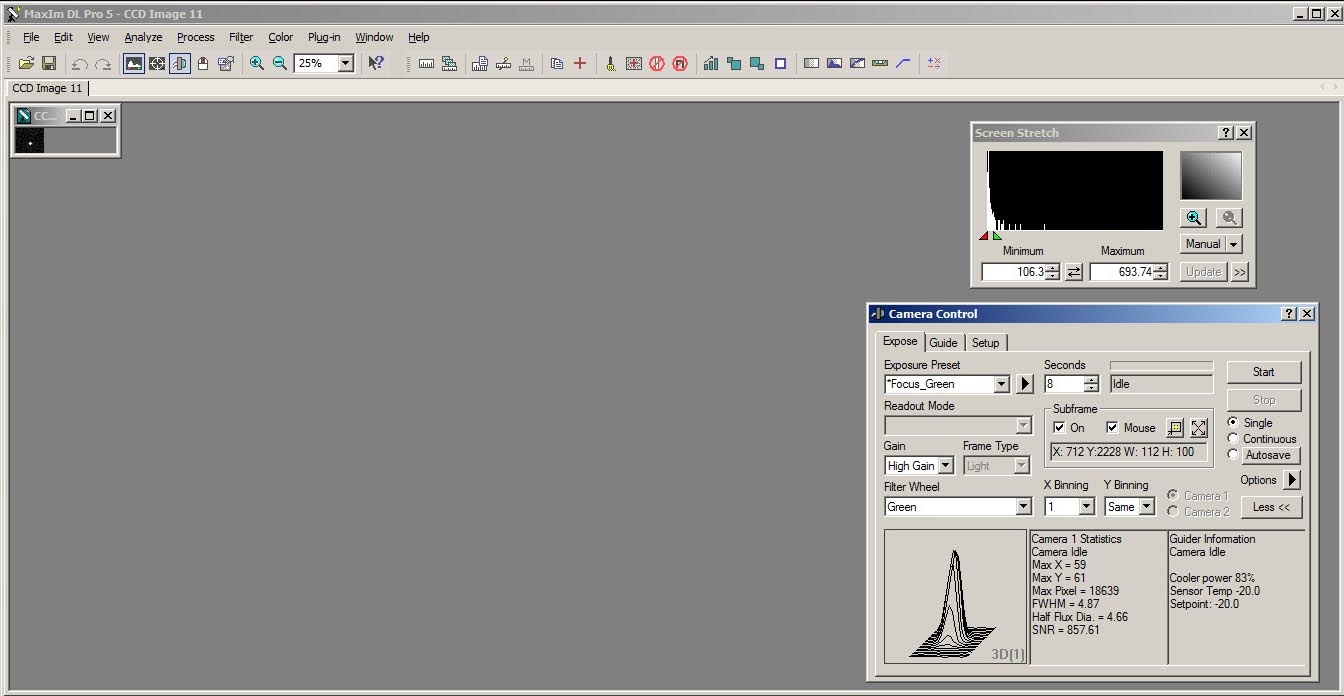
Figure 4. Example of the Information Window in the Maxim DL Camera Control panel displaying the maximum pixel value for an imaged star.
To determine k values for our observing session, we need two types of data: (1.) photon flux data for the imaged G2V stars, and (2.) elevation data for the imaged stars. The photon flux data were extracted from the images using AIP4WinV2. Other image processing software could probably be used for this task.
Extracting photon flux data from the images is a simple though somewhat tedious task. To do it, I use the Color Calculator tool in AIP4WinV2 (see Figure 1). The procedure for doing this is as follows.
(1.) Start AIP4WinV2 and open the Color Calculator tool (it's under the "Color" tab on the AIP4WinV2 toolbar).
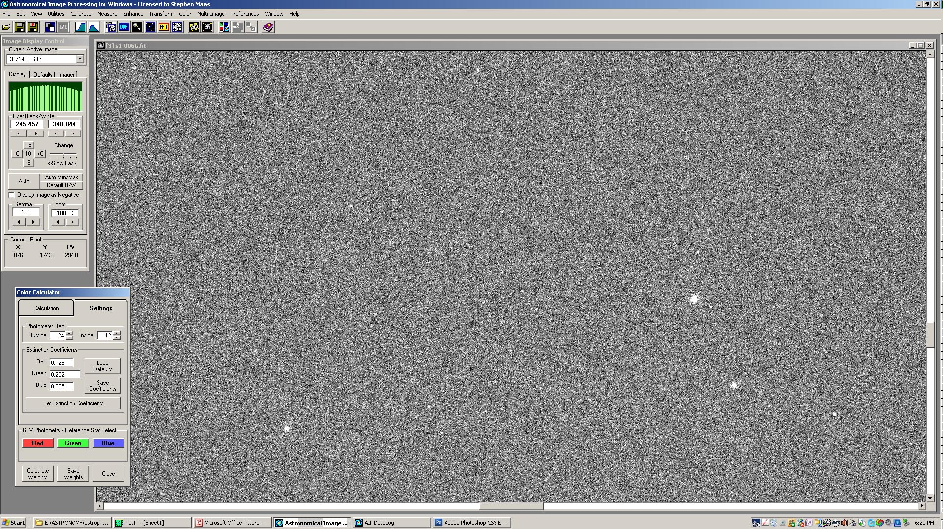
(2.) Open a color triad of images (one red, one green and one blue image) for one of the target stars. The computer screen should look something like Figure 5.
(3.) To measure the photon flux for the target star, we will use a photometric procedure in which we measure the photon flux of the star and then compare it to the photon flux of the starless region immediately surrounding the target star. To set up the tool for these measurements, go to the "Settings" tab in the Color Calculator tool. Note that, at this point, we can ignore the extinction coefficient values displayed on this tab— we won't be using them in our calculations. We'll need to set the sizes of the regions that will be used in our photometric measurements. This is done by specifying the "Photometer Radii" on this tab. When you open the tool, there will be default values displayed for the Outside and Inside Photometer Radii. These may or may not be good for our measurements. To check, click the cursor on the target star in one of the opened images. Then click one of the red, green, or blue buttons near the bottom of the tool (at this point, it doesn't matter which one). Two concentric circles will be drawn around the target star in the image. It should look something like Figure 6.
Figure 5. First step in extracting photon flux data using the Color Calculator tool in AIP4WinV2.
(4.) As shown in the figure, the area of the inner circle should completely enclose the target star in the image. It's okay for there to be a little open space between the star image and the circle. The radius of the second circle should be large enough so that the area of the annulus between it and the inner circle is at least as large as the area of the inner circle. However, it should not be so large that it encloses neighboring stars (like the small star next to the target star in the image). Adjust the values for the radii in the Color Calculator tool (clicking on one of the color buttons after each change to refresh the display) until you're satisfied with the results.
Figure 6. Establishing the photometer radii using the Color Calculator tool in AIP4WinV2.
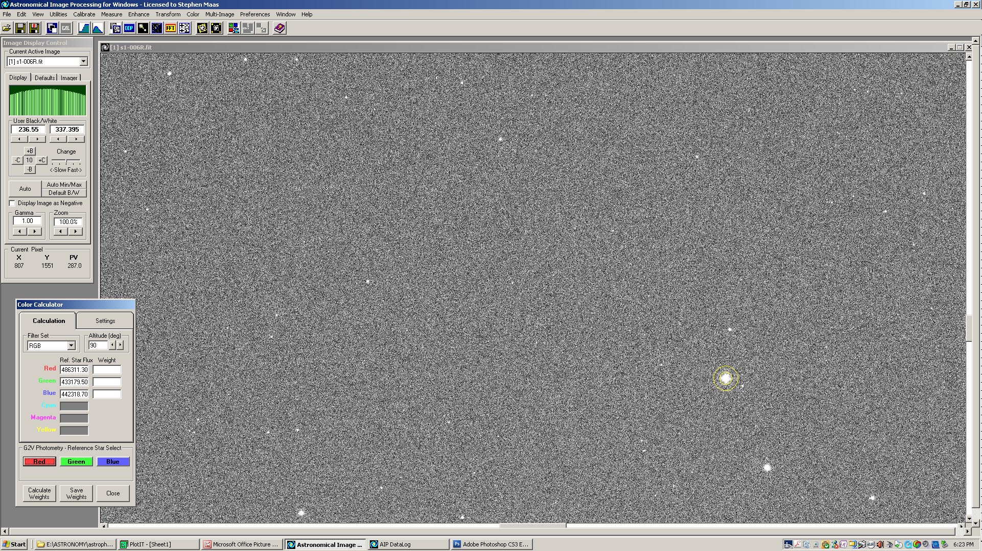
(5.) Once you've established the photometer radii, you're ready to start making photon flux measurements. Switch to the "Calculation" tab in the Color Calculator tool (see Figure 7). Make sure the "Filter Set" is RGB. Ignore the "Altitude" setting (we won't be using it at this point). Under "Ref. Star Flux" there may be some values in the red, green and blue boxes— these came from our earlier playing around with the photometer radii. We'll now get the correct values of the star fluxes. In the displayed images, click the cursor on the target star. Then click the appropriately colored button near the botton of the Color Calculator tool. For example, if you clicked the star in the green image, then click the green button. Do this for each of the three displayed images. When you click the star in an image and the appropriately colored button, photometer radii will be drawn around the star and the value of photon flux will appear in the appropriate "Ref. Star Flux" box, as shown in Figure 7.
(6.) Save the three photon flux values (red, green and blue) for later analysis. I like to save them in an Excel spreadsheet. Yes, you will need to manually type them into the spreadsheet (I warned you that this procedure was somewhat tedious).
Figure 7. Calculating the photon fluxes for the displayed red, green and blue images.
(7.) Repeat Steps 5 and 6 for each triad of red, green and blue images acquired for a target star. When you're finished with the star, your spreadsheet should look something like Figure 8, with three columns representing the photon flux values in the red, green and blue spectral bands. If you did a good job in establishing the photometer radii, you won't need to change them for each new image of a target star. You may need to change them when you go to another target star, due to differences in stellar magnitude. The resulting database will contain one photon flux measurement for each acquired image. For the example described earlier, the database will contain 210 values.
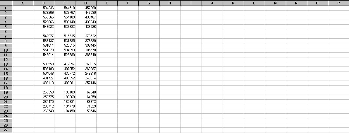
Figure 8. Portion of a spreadsheet showing the photon flux values for star #1 in the red (column B), green (column C), and blue (column D) spectral bands.
One great thing about this photometric approach is that you can do it on a moonlit night. Since the photon flux from the sky background (determined from the photometer outer annulus) is subtracted from the photon flux for the inner photometer circle containing the target star, the values presented in the Color Calculator tool are automatically calibrated for sky background brightness. This makes collecting data for determining atmospheric extinction coefficients a good thing to do on those bright moonlit nights when you can't effectively image anything else. Just be sure that the moon isn't right next to the target stars, where it's glare might completely wash them out. This feature also corrects for the presence of light domes near the horizon. What it doesn't correct for is differences in atmospheric transmissivity due to clouds or haze. It is sometimes difficult to detect the presence of thin cirrus clouds or dust (or pollution) haze in the night sky. These will affect the photometric measurements and result in "bad data." So, be sure that the night is really clear before attempting these measurements.
Another great thing about this procedure is that you don't need to apply dark frames to the acquired images. Since the effect of the sensor dark current is present in both the measurements of the star flux and the background flux, the values for photon flux presented in the Color Calculator tool are automatically calibrated for this effect. In addition, if you keep the target stars near the center of the acquired images, you can probably skip applying flat frames to the images.
Okay, we're halfway through our exercise. We need to determine the elevation angle above the horizon for the target star in each acquired image. We will later use this stellar elevation angle to calculate the optical thickness of the atmosphere through which we're observing the star. If your telescope mount is connected to your imaging computer, the elevation angle might automatically be included in the header of each image file. Otherwise, it's a simple (but, again, somewhat tedious) task to determine the stellar elevation angles.
The stellar elevation angle (SEA) can be manually determined from the image acquisition time. The acquisition time should be included in the header of each image file. Alternately, the time that the image file was written to the computer hard drive can be found from a listing of the image files (this time should be about the same as the image acquisition time, unless your computer is REALLY slow). I provide a computer application for calculating stellar elevation angle. Alternately, you can go into a planetarium software application (like Cartes du Ciel or Starry Night) and pick off the elevation angles for the target stars at the appropriate acquisition times. These values are enterred into the existing database. So, for each image acquisition, you will have values for red, green and blue photon fluxes and stellar elevation angle in the database. Your spreadsheet should now look something like Figure 9. Since the images for an RGB triad were acquired at about the same time, a single value of elevation angle (column F) has been entered in the spreadsheet for it. From this point on, the remaining tasks are just calculations using the data.
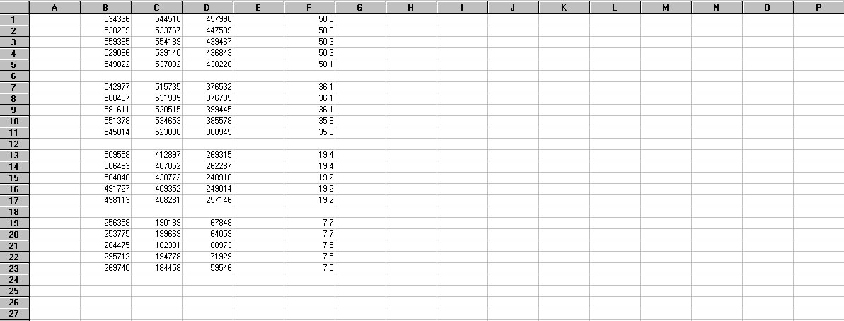
Figure 9. Portion of the spreadsheet from Figure 8 showing the elevation angle (column F, in degrees) associated with each RGB triad of photon flux measurements.
The first task is to calculate the optical thickness or "air mass" X through which we are observing the star. X is a function of the secant (reciprocal of the cosine) of the stellar zenith angle (SZA). SZA is the complement of the stellar elevation angle, so SZA = 90 - SEA (in degrees). Accounting for the curvature of the earth, X can be calculated as follows:
X = sec(SZA) - 0.0018167[sec(SZA)-1] - 0.002875[sec(SZA)-1]2 - 0.000808[sec(SZA)-1]3
If you're familiar with using Excel, these calculations can be done directly in the spreadsheet. Your spreadsheet should now look something like Figure 10. More details on the calculation and interpretation of X can be found in "The Handbook of Astronomical Image Processing" by Richard Berry and James Burnell (Willmann-Bell Publishers, Richmond, VA, 2009).
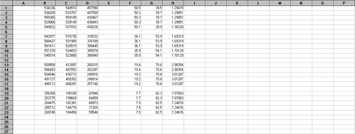
Figure 10. Portion of the spreadsheet from Figure 9 showing computed values of the stellar zenith angle (column G) and air mass X (column H).
The second task is to calculate the natural logarithm (base e) of the photon fluxes in the database. Stellar magnitudes are expressed on a logarithmic scale, so these calculations convert the photon fluxes into "magnitudes". We will call these magnitude values Ln(S), where S is the photon flux. These Ln(S) values are not the same as the actual visual magnitudes (like those shown in Table 1), but they could be converted into actual visual magnitudes through calibration based on reference stars. For determining atmospheric extinction coefficients, we don't need actual visual magnitudes. Figure 11 shows the spreadsheet with the computed values of Ln(S) in columns J, K and L.
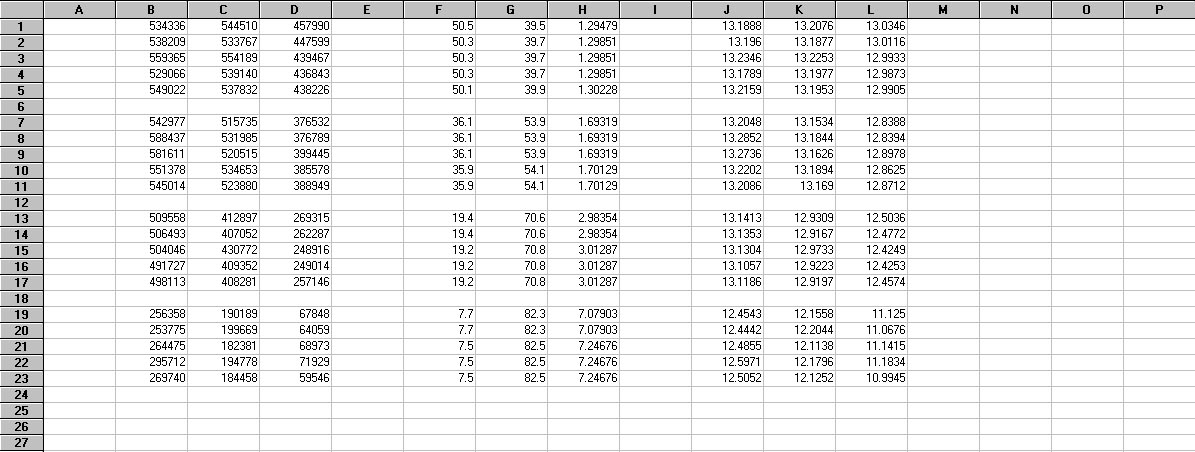
Figure 11. Portion of the spreadsheet from Figure 10 showing computed values of Ln(S) for the red (column J), green (column K), and blue (column L) spectral bands.
At this point, we can visualize our results by plotting Ln(S) versus X for the data in our database. This is shown in Figure 12 for the four stars in our example (Table 1). A separate graph is provided for each spectral band (blue, green and red). The graphs in Figure 12 were produced with a scientific graphing software application ("PlotIt") that I commonly use, but could be produced in Excel or other software packages.
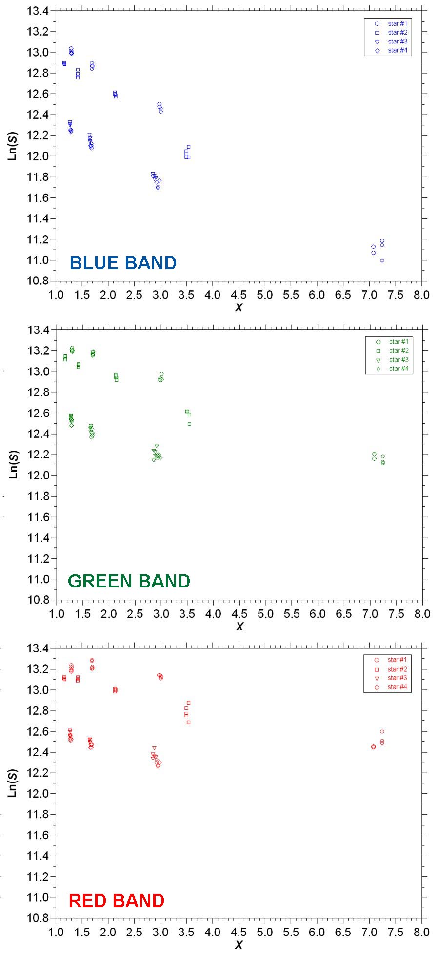
Figure 12. Ln(S) in the red, green and blue spectral bands plotted versus X for the stars in Table 1.
The data in Figure 12 behave as we would expect. Namely, as the air mass X increases (i.e., as the star gets closer to the horizon and its light has to pass along a longer optical path), the magnitude Ln(S) of the star decreases (i.e., the light from the star experiences more attenuation and scattering). In fact, the stellar magnitude should decrease exponentially with increasing air mass. In the graphs in Figure 12, an exponential decrease would be represented by a straight line with a negative slope. Based on this hypothesis, the data points for each target star in the red, green and blue spectral bands were fit with regular least-squares linear regressions (data for stars #3 and #4 were combined since they tended to cluster together). These regressions can be run within the Excel spreadsheet, or can be performed by other software packages. Theoretically, the slopes of these regressions within a given spectral band should be the same. Analysis showed that, in most cases, the slopes for this example were similar within a spectral band. As a result, the average of the slopes for each spectral band was calculated. For this example, the average slopes were -0.1380 (red), -0.2050 (green), and -0.3313 (blue). These average slopes were then used to determine contrained linear regressions (they were "constrained" in that all regressions for a given spectral band had the same slope) through the data points for each target star (again, the data for stars #3 and #4 were combined). The results of this operation are shown in Figure 13.
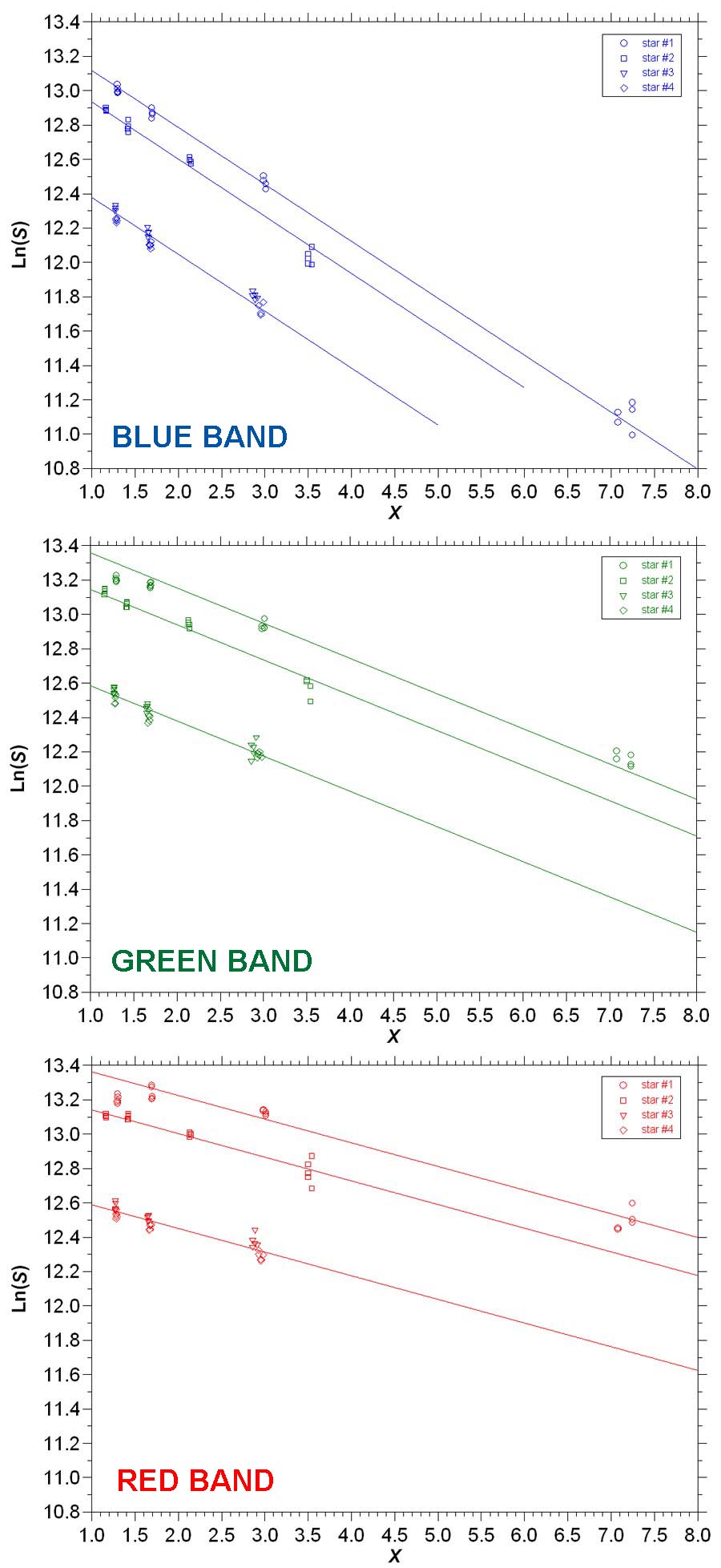
Figure 13. Constrained linear regressions between Ln(S) and X for the data in Figure 12.
In general, the constrained linear regressions fit the observed data points in Figure 13 quite well. This will usually be the case when you run this type of analysis, assuming you follow the instructions I've laid out for acquiring the image data. Occasionally, groups of data points will deviate from the straight lines. This can be caused by the passage of a thin cloud, or changes in overall atmospheric transmissivity during the course of the imaging session. Actually, it's not necessary that you plot the regressions like in Figure 13 to evaluate the extinction coefficients, but doing so provides a good check on the overall quality of the data and results.
After you've calculated the average regression slopes for the red, green and blue spectral bands as described above, YOU'RE FINISHED! This is because the values of the extinction coefficients for the red, green and blue spectral bands are numerically equal to the slopes of the regressions. Thus, for this example, kr = 0.1380, kg = 0.2050, and kb = 0.3313 (where the r, g and b subscripts denote the red, green and blue spectral bands). While the green value is reasonably close to the corresponding default value in Figure 1, the red and blue values are around 10% greater. Note that kb > kg > kr. This should always be the case, since shorter visible wavelengths of light are affected more by atmospheric transmissivity than longer visible wavelengths of light. In other words, the magnitude of the blue component of starlight falls off much more rapidly than the red component as the star moves down toward the horizon. However, now that you've got actual values of the extinction coefficients for your site, you can accurately correct your imagery for this effect.
In summary, determining atmospheric extinction coefficients is an easy task and is something that can be done on those moonlit nights when you can't do any other imaging. Atmospheric transmissivity is affected by factors that change from season to season, like humidity and wind (i.e., dust). Thus, you may want to evaluate extinction coefficients at different times during the year to capture these seasonal variations. Then, you could choose values for the extinction coefficients that could be applied to processing acquired astro-imagery based on the prevailing atmospheric conditions. As an ongoing project, I have been periodically collecting G2V star data at SOCO and calculating the resulting k values. Plotting the data versus date shows considerable variation in k over time, but analysis of these data indicates that most of the variation appears to be explained by changes in atmospheric moisture content.
Table 2 shows values determined for the atmospheric extinction coefficients from recent observing sessions at SOCO. The value for each date was derived from the data from four G2V stars. All observations were made on nights following cold front passages— skies were clear, temperatures were cold, and humidities were very dry. SOCO is around 1 km above sea level.
Table 2. Values for extinction coefficients from recent observations at SOCO.
|
For comparison, the default values in my copy of AIP4WinV2 are kr = 0.128, kg = 0.202, and kb = 0.295. In "The Handbook of Astronomical Image Processing" (Willmann-Bell Publishers, Richmond, VA, 2009), Richard Berry and James Burnell give the following values: kr = 0.13, kg = 0.20, and kb = 0.29 (for "moist, low-altitude observing sites"); and kr = 0.07, kg = 0.12, and kb = 0.22 (for "dry, high-altitude observing sites"). As you can see, there is considerable variability among reported values for atmospheric extinction coefficients, so it's best to just calculate your own.
So, you don't feel like going through all the laborious calculations described above to determine the values of atmospheric extinction coefficients? A new version (April 2022) of the Atmospheric Extinction Coefficient Calculator called "CAT-X" is now available that does all the calculations for you. All you need to run it is a set of FITS images of the target star in the red, green and blue spectral bands and some additional information (latitude and longitude of the observing site, and the RA and Declination of the target star). This makes calculating values of k very easy. You don't even have to use G2V stars for calculating extinction coefficients. If you do use G2V stars, CAT-X will also calculate weight factors from the image data. You can view the details for this application and download the executable file for it from the Cat-Star Astronomy Software Applications page of this website.
 Return to SOCO Image Processing Page
Return to SOCO Main Page
Return to SOCO Image Processing Page
Return to SOCO Main Page
Questions or comments? Email SOCO@cat-star.org