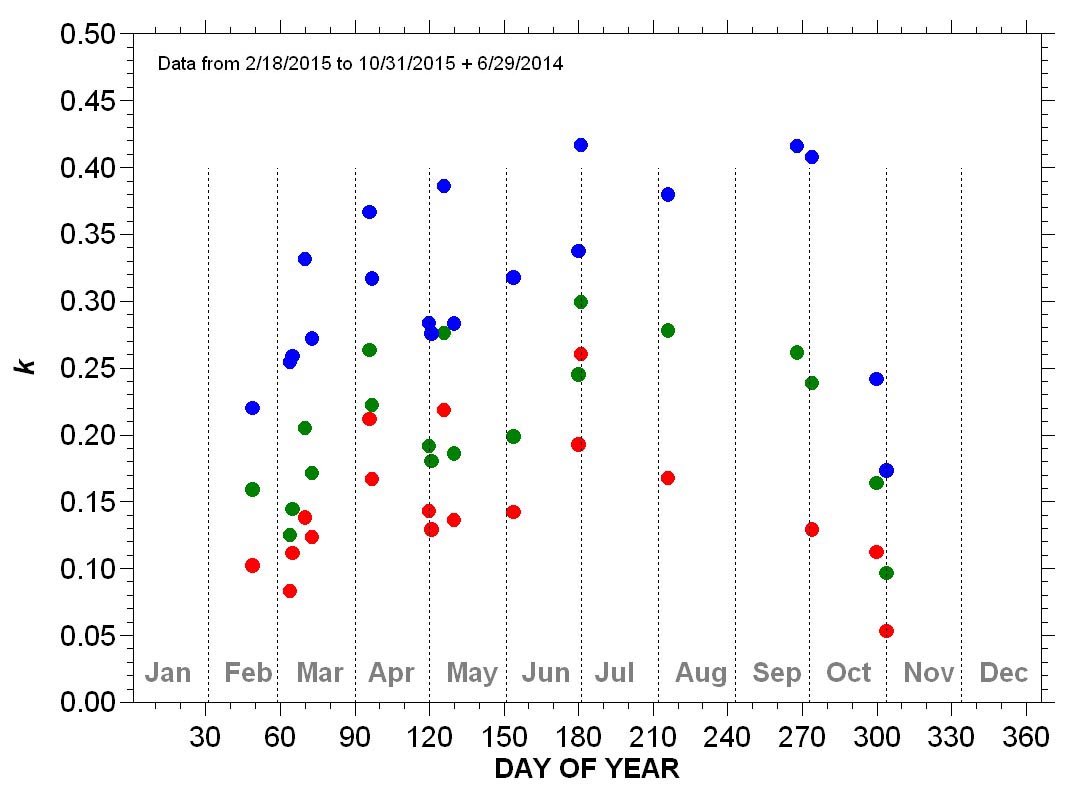
Figure 1. Values of kr (red dots), kg (green dots), and kb (blue dots) plotted versus day of year.
ATMOSPHERIC EXTINCTION COEFFICIENT CLIMATOLOGY
(April 2015)
(revised May 2015)
(updated July 2015)
(updated January 2016)
As an optical astronomer, I necessarily perform my observing and imaging activities on clear nights. Here in the Texas High Plains, the weather conditions that bring clear nights change over the course of the year. In the winter, it's the nights after the passage of cold fronts that produce the beautifully clear (and cold!) conditions. In the spring, dry southwest winds sweep away the clouds. And in the summer, it's the stable air mass conditions associated with the subtropical high pressure regions that give clear, warm, humid nights. Each type of weather has its own set of atmospheric conditions, including air temperature, humidity, wind and dust content, that potentially can affect the clarity of the atmosphere through which you're observing. In processing astronomical imagery, these effects are quantified through the values of the atmospheric extinction coefficient k. In another part of this website, I described in detail how to evaluate k for the red, green and blue spectral bands. Recognizing that the weather conditions that affect atmospheric clarity change over the year, I decided to investigate the degree to which k changes over the same time period. To address this topic, G2V stellar imagery were collected and evaluated for each month of 2015 during the period around full moon (weather permitting), when I normally wasn't doing any other astro-imaging. This should give a sufficient data set to determine to what degree k varies over the course of the year at this site— in essence, an extinction coefficient climatology. If the variation is sufficiently regular, it could serve as the basis for selecting k values for use in image processing as a function of time of year and/or prevailing weather conditions. Results of the project for the first year (2015) are presented in Figure 1. In addition to data collected this year, the figure contains one set of points collected at the end of June last year (2014). Apparent in the data is the transition from clearer Winter conditions (with lower k values) to Spring and Summer conditions characterized by an atmosphere with increasing humidity and aerosols (dust) and higher k values, and then a return to clearer conditions in the late Fall. The large gaps in the data set during August and September and again in November and December are the result of unusually cloudy conditions. The Fall of 2015 was characterized by "El Nino" conditions, which are usually associated with increased storminess in the American Southwest.
Results for 2015
Figure 1. Values of kr (red dots), kg (green dots), and kb (blue dots) plotted versus day of year.
So, what in the atmosphere is controlling the trend in k values? The results in Figure 2 give some indication. Here, k values from Figure 1 are plotted versus corresponding values of average dew point temperature (Td). The average dew point temperature was calculated for the period over which stellar G2V observations were made using data from a nearby weather station (Slaton, Texas), which is part of the West Texas Mesonet. Dew point temperature is a conservative measure of the amount of water vapor in the atmosphere. The data in Figure 2 suggest that the magnitude of k in all three spectral bands (red, green and blue) is significantly related to atmospheric moisture content.
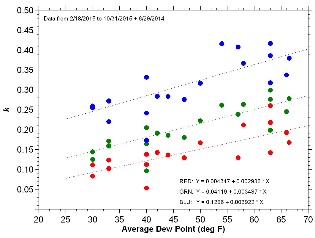
Figure 2. Values of kr (red dots), kg (green dots), and kb (blue dots) plotted versus average dew point (Td).
The data for the red, green and blue spectral bands in Figure 2 were fit with simple linear regressions. These regressions explained 59.6, 77.4, and 64.0 percent of the variance in the red, green and blue data sets, respectively. The slopes of the three regressions were significantly different from zero (at the 95% confidence level). This indicates that k values needed in processing astronomical imagery can be estimated with some degree of accuracy directly from measurements of Td obtained over the course of the imaging session, although the scatter in the points around each regression line suggests that possibly one or more as-yet undetermined atmospheric factors (such as aerosol content) may also be influencing the value of k.
A similar analysis can be performed for the weight factors used in processing imagery. Figure 3 shows the results of plotting the values of weight factors (W) for the red, green and blue spectral bands versus corresponding values of dew point temperature. These values were calculated using the procedure described for calculated weight factors assuming their equality at an air mass of 1 (i.e., X = 1). In this case, there was no apparent relationship between the weight factors for the red and green spectral bands and Td. However, the weight factor for the blue spectral band was observed to be weakly related to Td. We can summarize these results as follows:
W1,r = 1
W1,g = 0.9925
W1,b = 0.8717 - 0.001686 Td
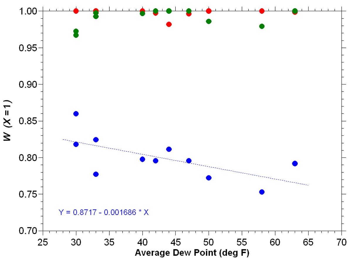
Figure 3. Values of W1,r (red dots), W1,g (green dots), and W1,b (blue dots) plotted versus average dew point (Td).
For Exoatmospheric G2V Correction, where the values of the red, green and blue weight factors are assumed equal outside the atmosphere (i.e., X = 0), the following results are provided:
W0,r = 0.9577
W0,g = 1
W0,b = 0.9654 - 0.001870 Td
If dew point data are not available, an average value for the blue weight factor W0,b = 0.8953 should be adequate for most image processing situations.
Values presented on this webpage will be updated as sufficient new data become available.
 Return to SOCO Image Processing Page
Return to SOCO Main Page
Return to SOCO Image Processing Page
Return to SOCO Main Page
Questions or comments? Email SOCO@cat-star.org