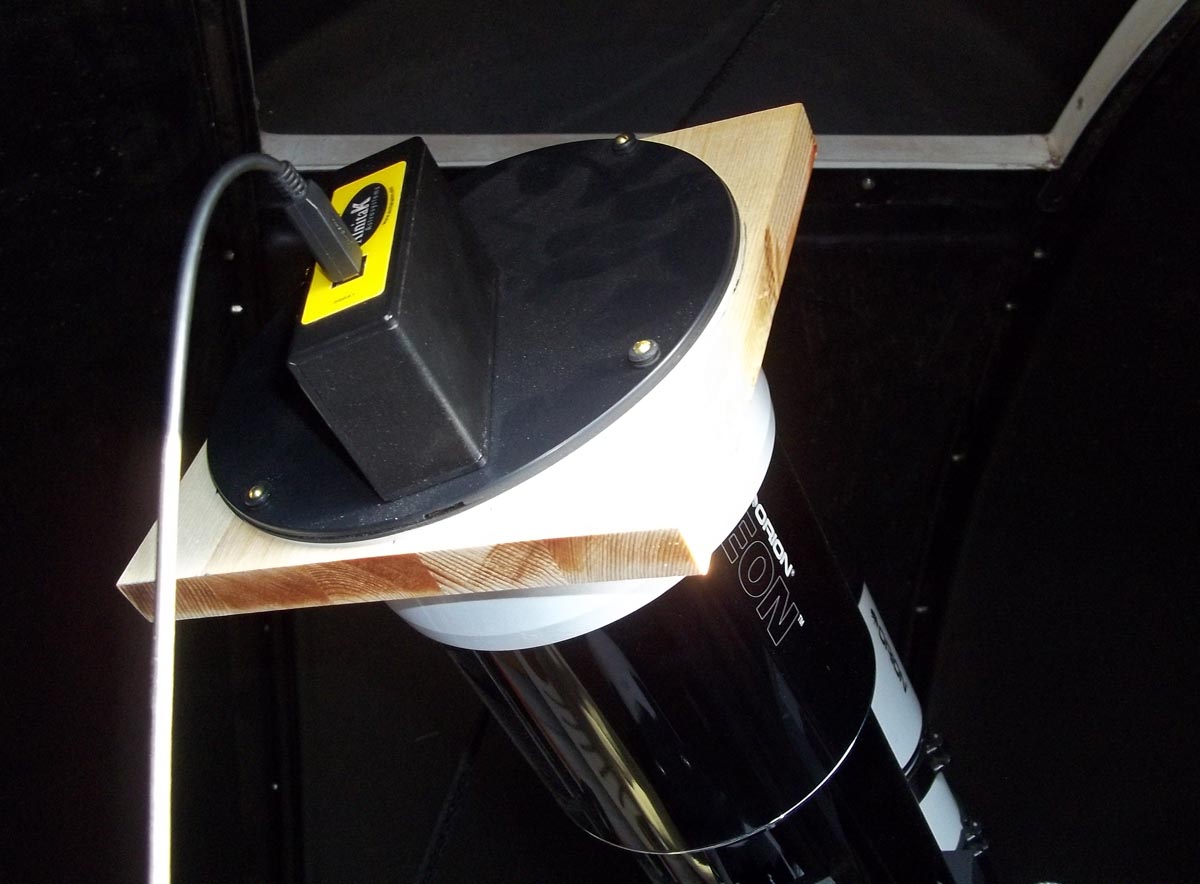
Figure 1. The Alnitak "Flat-Man" flat-fielding electroluminescent panel with custom-built holder.
MODELING FLAT IMAGES
(November 2015)
In working with the images produced by many imaging systems, one of the necessary processing steps is applying flat images (or "flat-field frames") to correct for optical artifacts in the images. The most common optical artifact is vignetting around the edges of the image. This is caused when the cone of light passing through the telescope does not uniformly illuminate the face of the CCD in the imaging camera. This could be because the cross-section of the cone of light focused onto the CCD is smaller than the dimensions of the CCD, or maybe there is a restriction in the optical path (e.g., from filters) at some point before the light reaches the CCD. In any event, the result is a marked fall-off of light along the edges (or in the corners) of the images. If this light fall-off can be quantified, then it is possible to apply a correction to the image during processing ro compensate for it. This will restore a more uniform brightness across the entire image. Flat images are specially shot images that can quantify the light fall-off. As described in the Handbook of Astronomical Image Processing (Richard Berry and James Burnell, Willmann-Bell Publishers, 2009), there are four basic ways to acquire flat images: light-box flats, dome flats, twilight flats, and sky flats. I won't go into the details of each but, in the past, I have relied on light-box flats in my image processing. Figure 1 shows my apparatus for acquiring light-box flats. It consists of an electroluminescent panel (manufactured by Alnitak Astrosystems) mounted in a home-made holder that fits over the end of the telescope. When current is applied to the electroluminescent panel, it emits a uniform level of light across its surface area. Taking an image of the illuminated panel through the telescope will show any light fall-off across the acquired image. The average of a number of individual flat images can then be used as a "Master Flat Image" to correct imagery acquired of astronomical objects, as I describe in Basic Processing Procedure I. This apparatus is easy to use and can be used at any time, day or night.
Figure 1. The Alnitak "Flat-Man" flat-fielding electroluminescent panel with custom-built holder.
In my astro-imaging, I use three optical systems: QSI digital camera alone (no additional optics between the telescope and camera), QSI camera mounted with an Optec 0.7X focal reducer, and QSI camera mounted with a TeleView 2X focal extender. Details of these optical systems are presented on the Astronomical Equipment page of this website. Examples of raw flat-field images acquired for each of these systems using the Alnitak electroluminescent panel are presented in Figure 2. In these images, the contrast has been compressed to emphasize the variation in brightness across the imaged field. Figure 3 shows graphs of the pixel digital count (DC) values along transects running diagonally from the upper left to lower right corners of each image (the thin white line in each image).
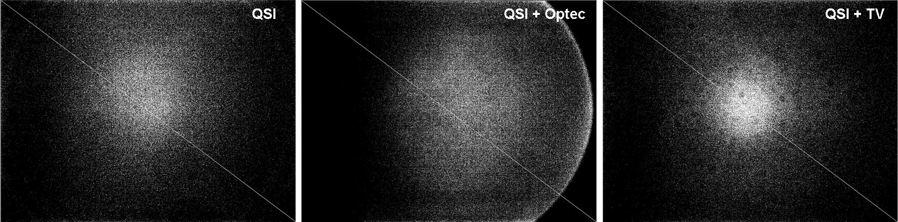
Figure 2. Flat-field images acquired for (left) the QSI camera alone, (middle) the QSI camera with Optec 0.7X focal reducer, and (right) QSI camera with TeleVue 2X focal extender.
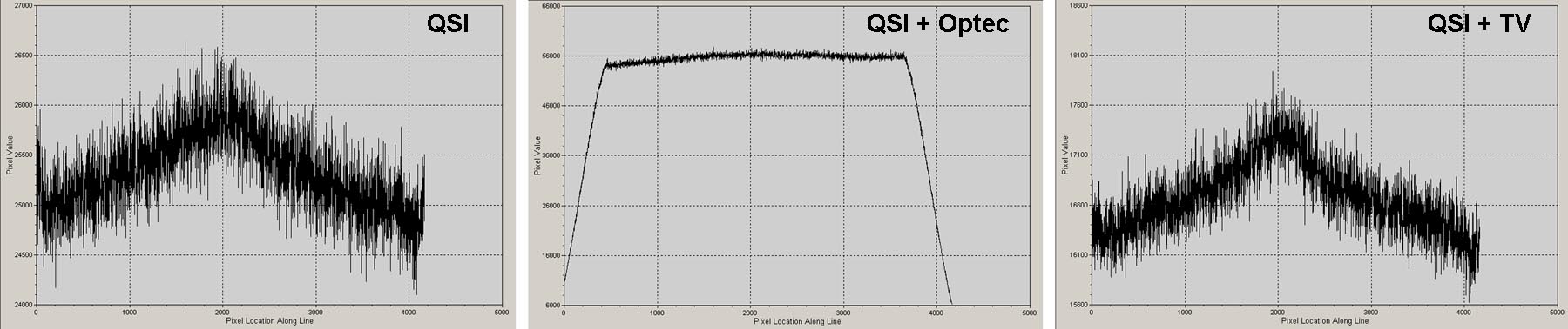
Figure 3. Graphs of pixel DC values along the diagonal transects indicated (thin white lines) in the images in Figure 2.
The results in Figures 2 and 3 show a central "hotspot" in the images for the QSI camera alone and the QSI camera with 2X focal extender. For both cases, the center-to-edge variation in brightness was around 1000 DCs. For the QSI camera with 0.7X focal reducer, the variation is more complex, with a central plateau in brightness rapidly falling away as the corners are approached. As the middle image in Figure 2 indicates, this plateau structure is not entirely symmetrical about the center of the image.
By acquiring and averaging a number of images like those in Figure 2, and then normalizing them by their average maximum (central) values, Master Flat Images can be produced for correcting for these apparent artifacts in the imaging systems. Until recently, this was the procedure I used in processing astronomical images at SOCO.
Figure 4 shows three raw light images (red band) acquired for various astronomical objects using the optical systems previously described. In each case, the target object does not occupy a large portion of the image. Also, each image was acquired when the target was high in the sky to avoid gradient effects near the horizon. Figure 5 shows graphs of pixel DC values along diagonal transects for these three images constructed in the manner of Figure 3. While the transects intersect a few stars (indicated by the spikes in DC values on the transects), they mostly show the variation in background sky brightness across an image.
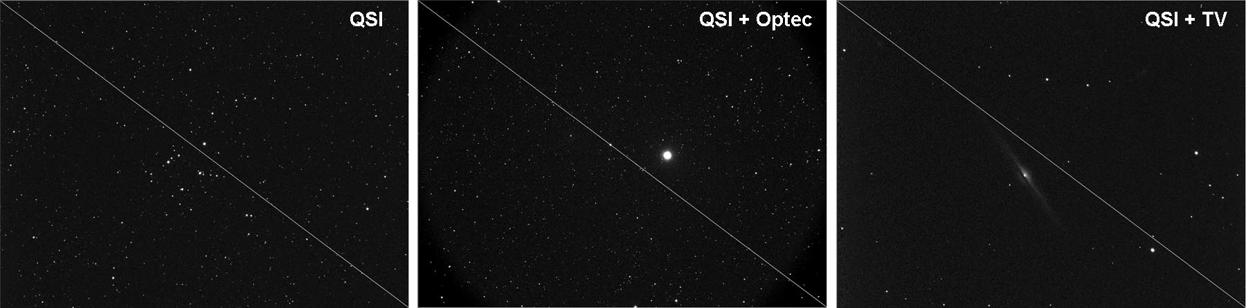
Figure 4. Raw light images acquired for (left) the QSI camera alone, (middle) the QSI camera with Optec 0.7X focal reducer, and (right) QSI camera with TeleVue 2X focal extender.
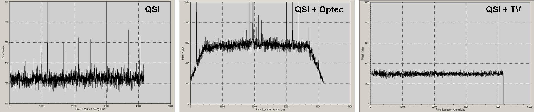
Figure 5. Graphs of pixel DC values along the diagonal transects indicated (thin white lines) in the images in Figure 4.
In viewing the graphs in Figure 5, one would expect the variation in background sky brightness across the images to be qualitatively similar to the corresponding graphs in Figure 3, since the sky within the field of view of the telescope is acting like a uniform emitter of light. What is immediately obvious, however, is that the graphs in Figure 5 for the QSI camera alone and the QSI camera with 2X focal extender do not exhibit any appreciable variation in brightness along the length of the transects above the random pixel-to-pixel variations. This is in stark contrast to the corresponding graphs in Figure 3, which show central "hotspots" in the images for these two systems. The graph for the QSI camera with 0.7X focal reducer in Figure 5 is somewhat similar to the corresponding graph in Figure 3, but the plateau-like structure in the graph in Figure 5 is symmetric about the center of the image (this symmetric nature has been verified by analyzing numerous raw light images of this type).
What I have concluded from considerable analysis of raw images is that use of the electroluminescent panel in its current setup is introducing additional brightness artifacts into the flat-fielding imagery. I am not certain how this is happening, but I would guess that it is related to the position of the source of illumination. The night sky as a source of illumination is very far from the aperture of the telescope, so light rays entering the telescope's optical path are roughly parallel. With the electroluminescent panel, however, the source of illumination lies at the aperture of the telescope, so that light rays entering the telescope's optical path from various locations on the surface of the electroluminescent panel are not necessarily parallel.
Based on these findings, I have re-evaluated my procedures for processing imagery. When using the QSI camera alone or the QSI camera with 2X focal extender, no correction for vignetting is applied to the imagery. Correction for vignetting is obviously needed when using the QSI camera with 0.7X focal reducer. However, the regularity of the brightness response across the image for this optical system made me wonder if a mathematical model could be constructed of it. If sufficiently accurate, this model could be applied to light imagery as part of the processing procedure without the need for actual flat images.
Numerous light images of relatively "blank" star fields (places in the sky away from the Milky Way with relatively few stars) were acquired using the QSI camera with the 0.7X focal reducer with exposure times ranging from 1 second to 900 seconds (15 min). This is somewhat similar to what is done to produce "sky flats", except in this case the objective was to collect data for modeling the vignetting effect for this optical system. Analysis of the variation in background sky brightness across the image field from this set of imagery showed that the vignetting effect is a well-behaved function of several parameters. It was determined that the variation in background sky brightness for this optical system (as seen in the example in Figurre 5) could be approximated by a central "plateau" segment that, near the edges of the image, abruptly falls away linearly. The slopes of the linear segments on each side of the plateau are the same. The height of the plateau segment in terms of DC is a function of overall sky background brightness, which is determined by the "instantaneous" sky brightness (related to the amount of atmospheric scattering at the time of imaging) and the exposure time. The top surface of the plateau is not flat but is parabolic, with the curvature of the parabola also a function of overall sky background brightness. This functional shape is radially symmetric about the center of the image, i.e., if you take the functional form inducated by the transect in Figure 5 and rotate it 180 degrees about the center of the image, you get the full 2-dimensional form of the function for the entire image.
The modeled form of the vignetting function is shown on the left side of Figure 6. As shown on the right side of Figure 6, when the function is properly evaluated, it closely matches the distribution of sky brightness pixel values from actual light images.
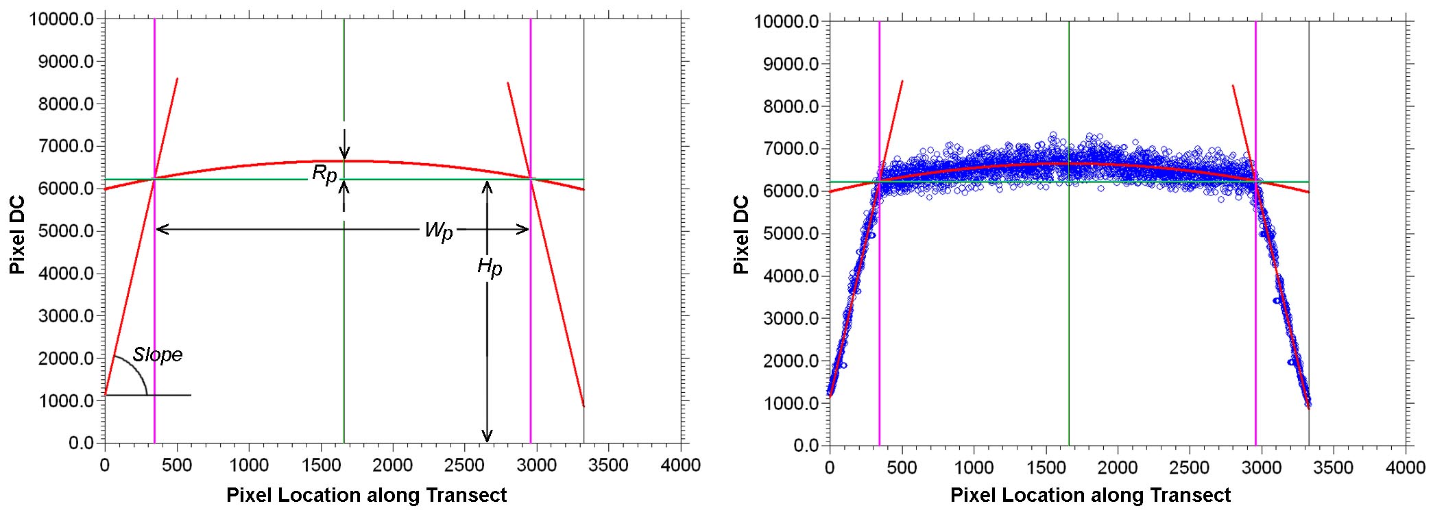
Figure 6. (Left) Modeled vignetting function (red lines); (Right) Fit of modeled function to image pixel DC data (blue circles).
Four parameters must be evaluated to construct the vignetting model (refer to Figure 6):
(1.) The width of the plateau section (Wp).
(2.) The height of the base of the plateau section (Hp).
(3.) The rise of the parabola above the base of the plateau section (Rp).
(4.) The slope of the sides of the function (Slope).
For a given spectral band (Red, Green, Blue, Hα, etc.), the value of Wp was found to be independent of sky background brightness in the image. The values of the other three parameters were found to increase with increasing sky background brightness in the image. Thus, the values of Hp, Rp, and Slope increased with increasing image exposure time (and to a lesser degree, decreasing atmospheric clarity). To apply this model to an astronimcal image, an estimate of the sky background brightness must be determined. However, this may be difficult to do with actual images of astronomical objects because the target object (like a nebula or galaxy) may occupy most of the central portion of the image, preventing the determination of sky background brightness in this portion of the image. However, I (like most astro-imagers) normally frame the target object in the image with some "blank sky" surrounding it. In this situation, a surrogate for the sky background brightness can be determined by calculating the median pixel brightness in each of the four corners of the image. I use a 25×25-pixel area to compute these median values (the median is used to remove the effects of stars that might lie in these areas). Lying in the very corners of the image, these small square areas rarely contain any of the target object. The average of these four median values is computed as a surrogate for sky background brightness.
Results of regressing the parameters Hp, Rp, and Slope onto corresponding values of average image corner pixel brightness are presented in Figure 7. These results are for the Red spectral band, but results for the other spectral bands are similar. As shown in Figure 7, the relationships between the parameters and image corner pixel brightness are very strong, with R2 values extremely close to 1. This confirms that image corner brightness should be effective in estimating the parameters in the vignetting model. These results were confirmed with additional data collected on other dates.
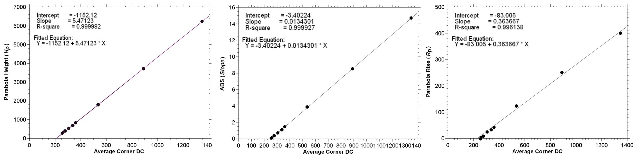
Figure 7. Regressions of parameters Hp, Rp, and Slope onto corresponding values of average corner pixel brightness for the Red spectral band.
One final feature that was added to the model was an empirical function that smoothes the transition from the plateau segment to the linear side segments. This is pretty much cosmetic, but makes the overall model match the image DC data even better. In practice, the model normally would be used to directly correct pixel values in the acquired light images during the image processing procedure. However, the model can be used to generate "synthetic" flat images. An example is presented in Figure 8.
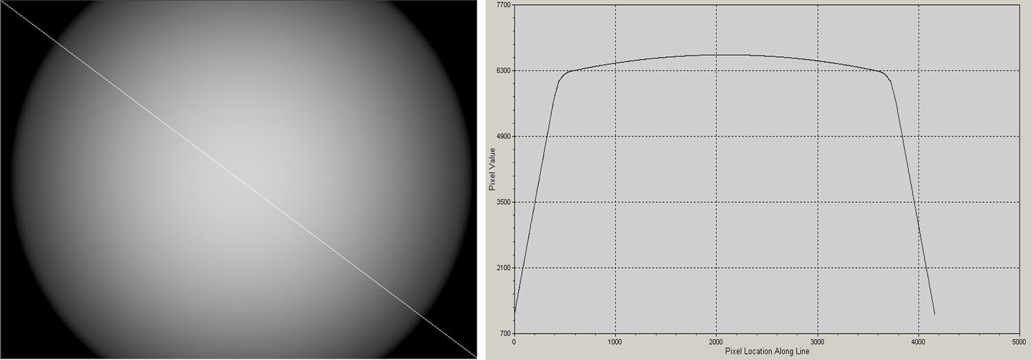
Figure 8. (Left) "Synthetic" flat image produced using the vignetting model; (Right) Pixel DC values along the diagonal transect in the image.
I've been using the flat field model for a couple of months now and I'm very pleased with its performance. It does as good or better a job at correcting vignetting effects in my imagery compared to flat images produced using the electroluminescent panel. This modeling procedure has been implemented in a new image processing program called SuperSIAM. Use of this automated modeling procedure has further simplified my image processing and removed the need to acquire flat images. It doesn't correct for "dust donuts" in the imagery, but these are a minor concern to me compared to the effects of vignetting.
 Return to SOCO Image Processing Page
Return to SOCO Main Page
Return to SOCO Image Processing Page
Return to SOCO Main Page
Questions or comments? Email SOCO@cat-star.org