Basic FITS Image Processing, Part II: Combining Broad-band (Red, Green, Blue) and Narrow-band (Hα, Hβ, OIII) Master Light Images
(August 2015) (supplemented November 2015)
Some astronomical objects present more of a challenge to image than others. Stellar objects, like open clusters, are easy— just a couple of minutes of exposure in Red, Green and Blue will capture about all the detail. Galaxies usually require high magnification and long exposures but, since they are basically just big collections of stars, they respond well to standard imaging in the Red, Green and Blue wavebands. The key is that stars are essentially blackbody emitters— they emit their energy over a continuous range of wavelengths as a function of temperature. Thus, imaging through broad-band Red, Green and Blue filters captures about all the visible light from them.
The biggest challenge involves trying to image emission nebulas— either HII regions like the Orion Nebula (M 42) or planetary nebulas like the Ring Nebula (M 57). These objects emit light as a result of electronic transitions at the atomic level— the resulting light is emitted in specific wavelengths that are characteristic of the electronic transitions. Unfortunately, the light emitted in these specific wavelengths is usually much dimmer than the light emitted across all wavelengths by stars. Thus, many emission nebulas are not very bright objects. You would need long exposures through broad-band Red, Green and Blue filters to adequately capture the light from these emission nebulas. Unfortunately, the stars in the same imaging field are generally putting out much more light across all visible wavelengths. So, what usually happens is that, for the nebula to be adequately exposed, the neighboring stars are over-exposed. The result is astro-images with big bloated stars that are not very attractive.
Luckily, you can now get narrow-band filters (at reasonable prices) that are "tuned" to the major emission wavelengths of nebulas. The three most common are Hα (656.3 nm), Hβ (486.1 nm), and OIII (500.7 nm). There are other emission wavelengths, but these three account for most of the light emitted by nebulas. Typical narrow-band filters have a band pass of only a few nm around these specific wavelengths, so they pass most of the nebular light while excluding light in other wavelengths. Since the light from stars is spread out over a broad range of wavelengths, only a small fraction is in the wavelengths passed by the narrow-band filters. This is ideally what we want— we can make long exposures through narrow-band filters and capture most of the light from the nebula while excluding most of the light from neighboring stars.
But there is a drawback to this. Images made solely through narrow-band filters show good detail in the nebula, but the stars in the image are subdued (many dimmer stars are entirely lost) so that the resulting image is unnatural in appearance— we count on the surrounding field of stars to act as a support for the nebula and provide depth to the image. Without surrounding stars, the nebula seems to float in the middle of nothing. What would be ideal would be to combine relatively short exposures through broad-band Red, Green and Blue filters (which show the star field nicely but not the nebula) with long exposures through narrow-band Hα, Hβ and OIII filters (which show the nebula nicely but not the stars). This can be done, but the trick is to come up with an objective procedure for combining the broad-band and narrow-band imagery that preserves the correct color balance and results in "true" color renditions of the object.
In Part II of this image processing procedure, I will describe a method that I have been working on to accomplish this. It makes use of Master Light Images in the Red, Green, Blue, Hα, Hβ and OIII wavebands created using the procedure described in Part I. The result is a set of "hybrid" Red, Green and Blue Master Light Images that can be combined into a composite "true" color image using the procedure described in Part III.
Relationship Between Broad-band and Narrow-band Filters
I currently use a set of Baader Red, Green and Blue filters in my imaging. The bandpass spectra for these filters are shown in Figure 1. The combination of these three broad-band filters pretty much covers the visible portion of the spectrum. Also shown in Figure 1 are the positions of the Hα, Hβ and OIII emission lines characteristic of nebulas. The positions of these emission lines relative to the bandpass spectra for the broad-band filters gives us some idea of how the imagery acquired with narrow-band Hα, Hβ and OIII filters might be combined with corresponding imagery acquired with broad-band Red, Green and Blue filters.
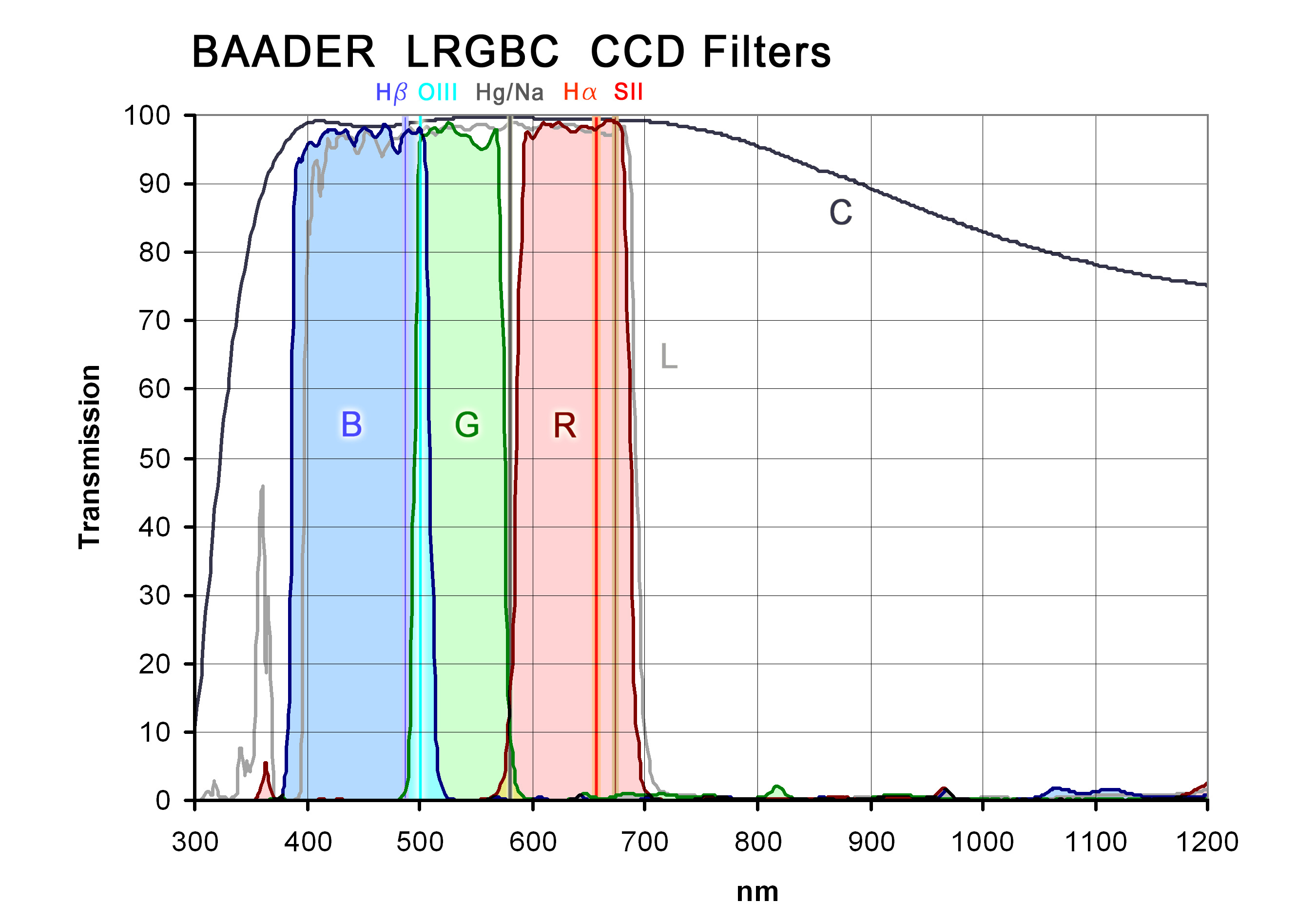
Figure 1. Bandpass spectra for Baader Red (R), Green (G) and Blue (B) filters and the positions of major nebula emission lines.
Source: Baader News 05/2008: "Baader announces Anti-reflective LRGBC filter-line to complement
Baader Narrowband CCD-Emission Line-filters".
First of all, the Hα emission line is completely contained within the spectral range of the Red broad-band filter. Thus, it would be logical to combine the imagery acquired with the narrow-band Hα filter with corresponding imagery acquired with the broad-band Red filter. Similarly, the Hβ emission line is completely contained within the spectral range of the Blue broad-band filter. Thus, it would be logical to combine the imagery acquired with the narrow-band Hβ filter with corresponding imagery acquired with the broad-band Blue filter. Dealing with the imagery acquired with the OIII narrow-band filter is a bit more complicated. Most broad-band Blue and Green astronomical filters are constructed so that their bandpass spectra overlap at around 500 nm. Thus, the light emitted in the OIII wavelength is equally captured in the broad-band Green and Blue images. This is intentional, because mixing equal amounts of green and blue light results in the "teal" color often attributed to OIII emissions, particularly from planetary nebulas. So, it would be logical to combine the imagery acquired with the narrow-band OIII filter with corresponding imagery acquired with the broad-band Green filter and also with the broad-band Blue filter. Thus, The broad-band Blue imagery would be combined with the imagery acquired with two narrow-band filters— Hβ and OIII. The broad-band Red imagery would be combined with the narrow-band Hα imagery, while the broad-band Green imagery would be combined with the narrow-band OIII imagery.
Combining Images Using Star Equalization
As simple as this seems, you can't just add the photon fluxes in the appropriate broad- and narrow-band images to produce a new Master Light Image. The images need to be combined in a way that maintains the same relative illumination levels among the resulting "hybrid" broad-band Red, Green and Blue Master Light Images as were in the original broad-band Red, Green and Blue Master Light Images. Otherwise, the color balance of the composite color image created from the new Master Light Images will be messed up and, in particular, the stars won't be the correct colors.
Luckily, there are features within the imagery that can be used as a guide to maintaining the correct relative illumination levels among the three Master Light Images— the stars themselves. In the remainder of this section, I outline a procedure for using measurements of the photon fluxes from stars in the imagery to equalize the relative illumination levels among the images being combined to produce "hybrid" Master Light Images that have the correct color balance.
Basic assumptions for this procedure are as follows:
(1.) All three broad-band (Red, Green and Blue) Master Light Images have the same exposure time.
(2.) All three narrow-band (Hα, Hβ and OIII) Master Light Images have the same exposure time.
(3.) The exposure time for the narrow-band Master Light Images was much longer than the exposure time for the broad-band Master Light Images.
Through trial and error, I have found that (with my telescope, camera and filters) I should expose the narrow-band images around 10 times longer than the broad-band images. For example, a 1.5-minute exposure is usually good for showing the stars in the image. Thus, I should use around a 15-minute exposure for the narrow-band images. In the resulting narrow-band images, the nebula is usually well-exposed, while the neighboring stars are still under-exposed. This is what we want. Our objective will be to create "hybrid" Red, Green and Blue Master Light Images in which the stars come from the original short-exposure broad-band images (Red, Green and Blue) and the nebula comes from the long-exposure narrow-band images (Hα, Hβ or OIII). The broad- and narrow-band images will be combined in a way that insures that the resulting set of "hybrid" Master Light Images has a similar color balance as the original set of broad-band Master Light Images.
The Procedure
To illustrate this procedure, I'll use imagery acquired for the Trifid Nebula (M 20) in Sagittarius. M 20 is a fairly bright emission nebula, but it is good for this example in part because we generally know what it is supposed to look like (color-wise). It also has a good mix of Hα, Hβ and OIII emissions (that give it that "electric pink" color), and it has an adjacent reflectance nebula that we can use (along with the stars) to judge how well the procedure maintains the proper color balance in the color composite image constructed from the hybrid images.
1. Create Master Light Images.
Master Light Images should be created for each spectral band (Red, Green, Blue, Hα, Hβ, and OIII) from the sets of raw light images using the procedure outlined in Part I. For this example, this will result in six Master Light Images: a broad-band Red image (IMGR), a broad-band Green image (IMGG), a broad-band Blue image (IMGB), a narrow-band Hα image (IMGHα), a narrow-band Hβ image (IMGHβ), and a narrow-band OIII image (IMGOIII).
2. Use the Image Math Tool in AIP4WinV2 to create a new Master Light Image by adding the Hβ and OIII Master Light Images.
As described previously, the broad-band Blue image contains two narrow-band emission features— Hβ and OIII (see Figure 1). To create a narrow-band equivalent of the broad-band Blue image, we need to add the pixel values for the Hβ and OIII images to create a new Master Light Image:
IMGHβ+OIII = IMGHβ + IMGOIII
Use the Image Math Tool in AIP4WinV2 (or a similar tool in other image processing software packages) to add the two images:
Open the Hβ and the OIII Master Light Images.
Add the Hβ and the OIII Master Light Images:
Multi-Image > Image Math�
An Image Math box will appear. Select the Hβ Master Light Image for A and the OIII Master Light Image for B. Select �Plus A+B� for the math operation. Click the �Perform Math Operation� button.
Save the resulting Hβ+OIII Master Light Image.
Close all opened files.
3. Collect Stellar Photon Flux Data from the Master Light Images.
Use the Single Star Photometry Tool in AIP4WinV2 (or a similar tool in other image processing software packages) to collect photon flux data for a common set of stars from each of the following Master Light Images: the broad-band Red image (IMGR), the broad-band Green image (IMGG), the broad-band Blue image (IMGB), the narrow-band Hα image (IMGHα), the narrow-band OIII image (IMGOIII), and the narrow-band Hβ+OIII image (IMGHβ+OIII). These six images are chosen because:
The narrow-band Hα image (IMGHα) corresponds to the broad-band Red image (IMGR)
The narrow-band OIII image (IMGOIII) corresponds to the broad-band Green image (IMGG)
The narrow-band Hβ+OIII image (IMGHβ+OIII) corresponds to the broad-band Blue image (IMGB)
The narrow-band Hβ image (IMGHβ) in itself doesn't correspond to any of the broad-band images, so it can be ignored for the remainder of the image processing. It's effect on the broad-band Blue image (IMGB) is contained in the narrow-band Hβ+OIII image (IMGHβ+OIII).
An example of using the Single Star Photometry Tool in AIP4WinV2 to collect stellar photon flux data is shown in Figures 2 and 3. First, open one of the Master Light Images. Then select "Measure" from the AIP4WinV2 Toolbar. In the drop-down list, select "Single Star Photometry Tool (SSPT) ...". The Single Star Photometry box will open. Select the "Settings" tab in this box— this will allow you tp specify the radii of the photometer rings that will appear in the opened image. Type in values for the radii of the inner and outer photometer rings and then click on a star in the image— a set of rings will appear around the selected star (Figure 2). If necessary, change the values for the radii until they fit the star properly (i.e., the inner ring is just larger than the star, while the outer ring does not contain any other stars). You will have to click the star after each time you change the radii values for them to take effect.
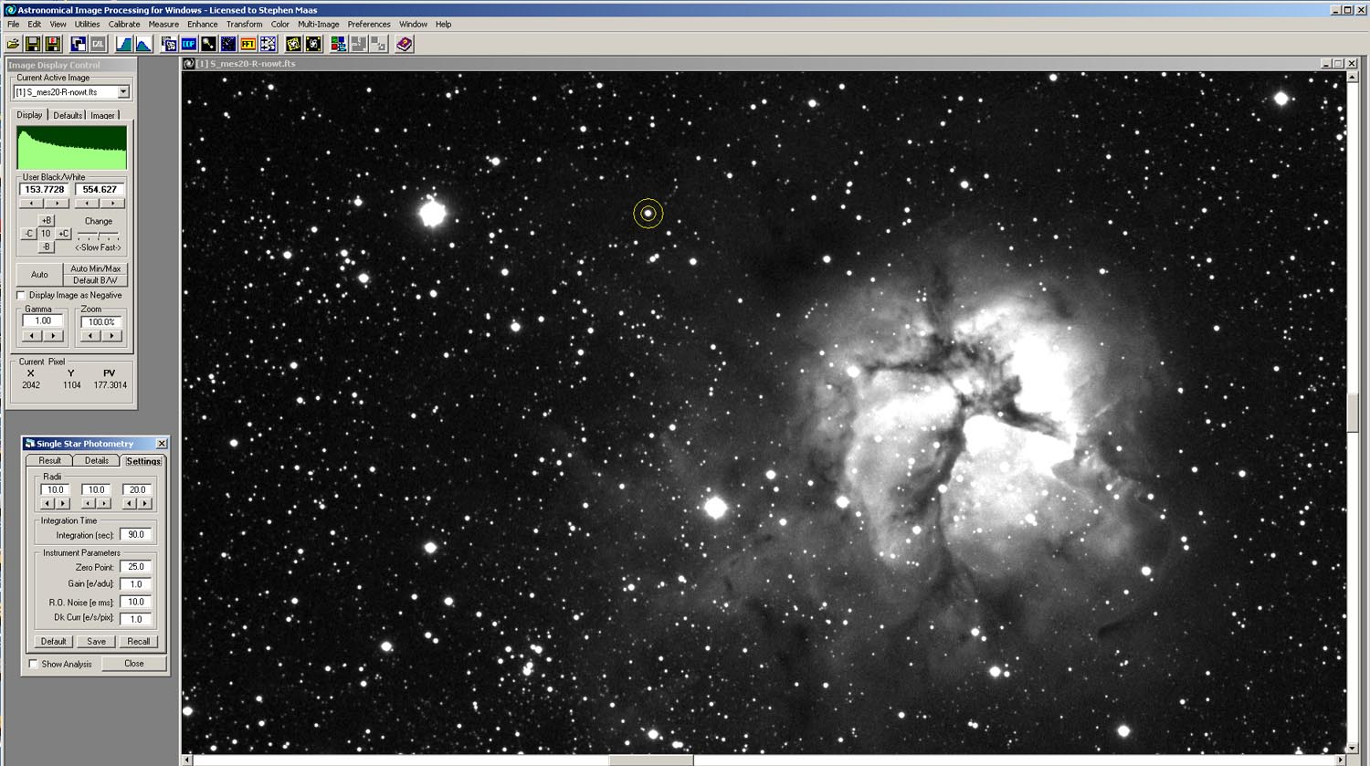
Figure 2. Setting the photometer radii for the Single Star Photometry Tool in AIP4WinV2.
Once you're satisfied with the photometer radii, select the "Result" tab in the Single Star Photometry Tool box. This will show the photon flux data for the star (Figure 3). Record the value for "Star - Sky" in the "Signal (in ADUs)" section of the box. Repeat this procedure for the same star in each of the six Master Light Images. Using this procedure, collect photon flux data for several stars (5 or 6 is good) in each Master Light Image. In selecting stars, choose medium-brightness stars in the images— not the brightest stars or the dimmest stars.
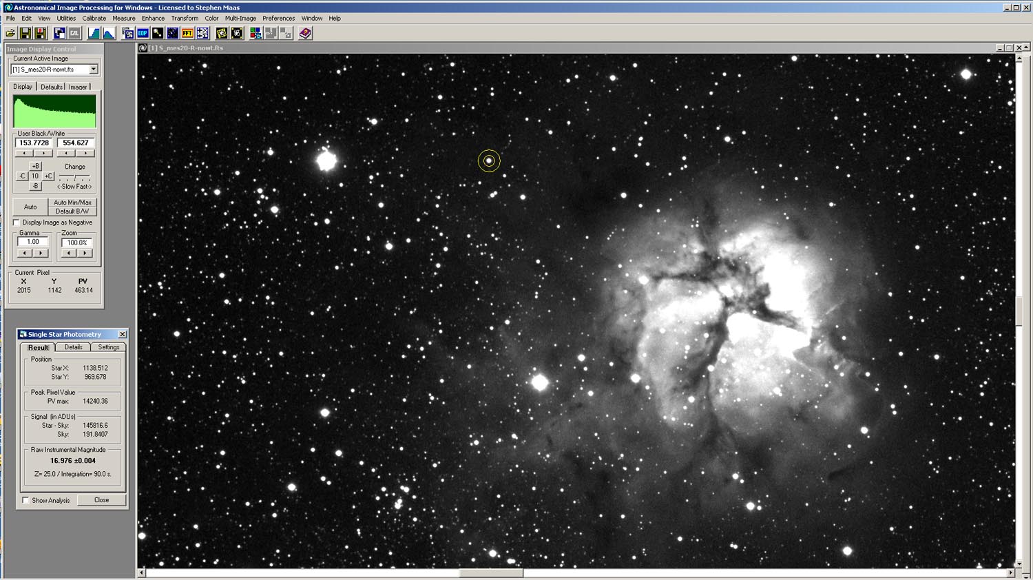
Figure 3. Photon flux data for the selected star.
After you've finished collecting data, calculate the average of the photon flux values for the measured stars from each of the six Master Light Images. Thus, you'll have one average photon flux value for each of the broad-band Red (IMGR), broad-band Green (IMGG), broad-band Blue (IMGB), narrow-band Hα (IMGHα), narrow-band OIII (IMGOIII), and narrow-band Hβ+OIII (IMGHβ+OIII) images— six values in all. For my example involving M 20, the results are shown in column 2 of Table 1. I've also included average photon flux values for a bright part of the nebula (determined using the "Information" Tool in Maxim DL in "Area" mode) in column 4.
Note— if the average nebula photon flux value for any of the narrow-band images is very small (i.e., close to the background brightness level), then you can probably omit that band entirely in processing the set of images. So, if the nebula is not putting out an appreciable amount of emissions in a particular narrow band, just ignore that band. For example, if the Hβ emissions were very small, then the Hβ+OIII image would consist of only the OIII image. If both the Hβ and OIII emissions were very small, then you'd only be concerned with combining the Red and Hα Master Light Images.
Table 1. Photon flux data for the example involving the Trifid Nebula (M 20).
| Spectral Band
| Average Stellar Photon Flux
| Ratio of Stellar Photon Fluxes
| Average Nebula Photon Flux
|
| Red
| 763663
|
| 589
|
| Green
| 560953
|
| 357
|
| Blue
| 413558
|
| 367
|
| Hα
| 519267
| Red/Hα = 1.4707
| 2561
|
| OIII
| 450399
| Green/OIII = 1.2455
| 588
|
| Hβ+OIII
| 791672
| Blue/(Hβ+OIII) = 0.5224
| 1044
|
Looking at the data in Table 1, we can see that the average nebula photon flux for the Hα band is greater than the corresponding value for the Red band (2561 > 589), the average nebula photon flux for the OIII band is greater than the corresponding value for the Green band (588 > 357), and the average nebula photon flux for the Hβ+OIII band is greater than the corresponding value for the Blue band (1044 > 367). This is what we wanted— the nebula is brighter in the longer-exposure narrow bands than in the corresponding shorter-exposure broad bands. Now, if the average stellar photon flux for the Hα band is less than the corresponding value for the Red band, the average stellar photon flux for the OIII band is less than the corresponding value for the Green band, and the average stellar photon flux for the Hβ+OIII band is less than the corresponding value for the Blue band, this would indicate that the stars are brighter in the shorter-exposure broad bands than in the corresponding longer-exposure narrow bands— this is also what we wanted. If this is the case, we could combine the pair of Red and Hα images, the pair of Green and OIII images, and the pair of Blue and Hβ+OIII images using a maximizing function to produce three new "hybrid" Red, Green and Blue Master Light Images:
HIMGR = Max [ IMGR, IMGHα ]
HIMGG = Max [ IMGG, IMGOIII ]
HIMGB = Max [ IMGB, IMGHβ+OIII ]
The maximizing function will compare a pair of images on a pixel-by-pixel basis and keep the greater value for each pixel. Thus, if the stars are brighter in the broad-band images than in the narrow-band images, then the stars in the resulting hybrid images will come from the broad-band images. Similarly, if the nebula is brighter in the narrow-band images than in the broad-band images, then the nebula in the resulting hybrid images will come from the narrow-band images. This was our objective in this processing procedure.
Looking at the data in Table 1, we see that the average stellar photon flux for the Red band is greater than the corresponding value for the Hα band (763663 > 519267), and the average stellar photon flux for the Green band is greater than the corresponding value for the OIII band (560953 > 450399). Unfortunately, after adding the Hβ image and the OIII image to produce the Hβ+OIII image, we find that the average stellar photon flux for the Blue band is not greater than the corresponding value for the Hβ+OIII band (413558 < 791672). As shown in column 3 of Table 1, the stars in the Blue image are only about half as bright as the stars in the Hβ+OIII image. If we perform our maximizing function on this pair of images, the stars and the nebula in the resulting hybrid Blue image will both come from the narrow-band Hβ+OIII image. This will throw off the color balance of the stars in a color composite image created from the hybrid Red, Green and Blue images because the exposure time for the stars in the Red and Green bands (which came from the shorter-exposure broad-band Red and Green images) is different from the exposure time for the stars in the Blue band (which came from the longer-exposure narrow-band Hβ+OIII image).
Don't worry— if this occurs, there is an easy fix for this! This fix is outlined in the next section.
4. Adjust the Stellar Photon Flux values using the Pixel Math Tool in AIP4WinV2.
Column 3 in Table 1 shows the ratios of the corresponding pairs of broad- and narrow-band Master Light Images. Note that, if all three of these ratios are greater than or equal to 1, you can skip this step in the procedure. For this example involving M 20, we are going to adjust the stellar photon fluxes in all three of the broad-band Master Light Images (IMGR, IMGG, and IMGB) according to the smallest value of the ratios (Rmin) in Table 1 (in this case, Rmin = 0.5224):
IMGR ← IMGR / Rmin
IMGG ← IMGG / Rmin
IMGB ← IMGB / Rmin
As indicated above, the old versions of the three images will be replaced in our processing by the new adjusted versions. Again, all three broad-band images (Red, Green and Blue) must be divided by the same ratio to maintain the proper color balance among them. Multiplying or dividing the three images by the same factor doesn't add any new information to them— it just moves their pixel values up or down the brightness scale by a proportional amount. With regard to our image processing, what it will do is make the stars in the broad-band images as bright ot brighter than the stars in the corresponding narrow-band images. Then, when we perform our maximizing function on the pairs of images, the stars in the resulting hybrid images will come from the respective broad-band images.
This image adjustment is performed using the Pixel Math Tool in AIP4WinV2 (or a similar tool in other image processing software packages):
Open one of the broad-band Master Light Images (Red, Green or Blue).
Open the "Pixel Math" tool:
Enhance > Pixel Math...
In the Pixel Math box, type in the value for Rmin in the space provided.
Among the button representing Math Functions, click the one labelled "pv/A".
Save (over-write) the resulting adjusted image.
Repeat this procedure for all the broad-band Master Light Images.
One potential problem may arise when you do this. When you adjust the broad-band Master Light Images, you increase the values of all the pixels in the images— not only pixels representing stars but also pixels representing the nebula. If the value of Rmin is too small, the photon flux values representing the nebula in one or more of the broad-band images might be increased so that they are now greater than the corresponding values for the nebula in the narrow-band images. When we perform our maximizing function, pixel values for the nebula in the resulting hybrid images might come from the broad-band images rather than the narrow-band images. This could potentially throw off the color balance of the nebula. In practice, this is not as much of a problem as potential color imbalances in the stars. This is because the average photon flux values for the nebula are much smaller than those for the stars in the imagery (generally by three or more orders of magnitude). Dividing by Rmin has a much smaller absolute effect on pixels representing the nebula than on pixels representing stars and, thus, has a much smaller effect on the color balance of the nebula. So, the color balance of the nebula should be relatively accurate even if some of the pixels represeting the nebula come from the broad-band images rather than the narrow-band images. This problem is more likely to show up in imagery of relatively bright nebulas. It should be minimal in imagery of relatively dim nebulas, which may not show up at all in the short-exposure broad-band images. Of course, you probably don't need to acquire narrow-band imagery of nebulas that are bright enough to be adequately imaged in the normal Red, Green and Blue bands (like our example of M 20).
5. Create Hybrid Red, Green and Blue Master Light Images using the maximizing function in Maxim DL.
At this point, we've got a set of six Master Light Images consisting of a broad-band Red image (IMGR), a broad-band Green image (IMGG), a broad-band Blue image (IMGB), a narrow-band Hα image (IMGHα), a narrow-band OIII image (IMGOIII), and a narrow-band Hβ+OIII image (IMGHβ+OIII). We're ready to combine them using the maximizing function described earlier to produce a set of three hybrid Master Light Images (HIMGR, HIMGG and HIMGB) that can be combined to produce a color composite image. To combine pairs of images using the maximizing function, we will use the Pixel Math tool in Maxim DL (as best as I can tell, AIP4WinV2 does not allow images to be combined using a maximizing function):
Open an appropriate pair of Master Light Images (IMGR and IMGHα, IMGG and IMGOIII, or IMGB and IMGHβ+OIII) in Maxim DL.
Open the "Pixel Math" tool:
Process > Pixel Math...
In the Pixel Math box, select one of the pair of images for "Image A".
In the "Operation" section of the box, click "Maximum".
Select the second image in the pair for "Image B".
Make sure the Scale Factors are 100% and the "Add Constant" value is zero.
Click the "OK" button. The image identified as "Image B" will be replaced with the new maximized version.
Save the resulting maximized image with a new name (don't over-write Image B).
Repeat this procedure for the two ther pairs of Master Light Images.
These hybrid Red, Green and Blue images can be treated like any other set of Red, Green and Blue Master Light Images. They can be used as inputs to Basic FITS Image Processing, Part III to produce a "true-color" color composite image.
Results
The results of our image processing exercise for M 20 are presented in Figure 4. The left side of the figure shows the color composite image created from the hybrid Red, Green, and Blue Master Light Images (HIMGR, HIMGG and HIMGB) using Basic FITS Image Processing, Part III. For comparison, the right side of the figure shows the corresponding color composite image created from the regular broad-band Red, Green, and Blue Master Light Images (IMGR, IMGG and IMGB), also using Basic FITS Image Processing, Part III. Similar amounts of contrast-stretching were applied to both images to produce the final versions presented in Figure 4.
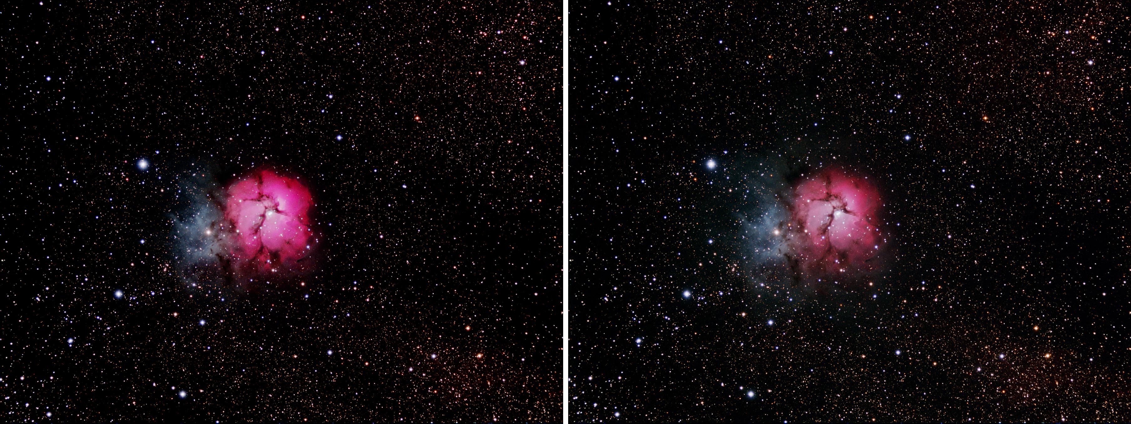
Figure 4. Color composite images of M 20 created using (left) Hybrid Red, Green and Blue Master Light Images, and (right) regular broad-band Red, Green and Blue Master Light Images.
In comparing the two versions of the color composite image, we can see that the stars surrounding the nebula are essentially the same (in terms of abundance, magnitudes, and colors) for both versions. This verifies that the stars in both versions came from the broad-band Red, Green and Blue images. The bluish reflection nebula along the left side of the main nebula body of M 20 is also the same in both versions of the color composite image. Thus, our manipulation of narrow-band emission images did not affect the appearance of the reflection nebula. The obvious difference lies in the representation of the emission portion of M 20. While the overall color ("electric pink") of the emission nebula is similar in the two image versions, the color in the version created using the hybrid Red, Green, and Blue Master Light Images (left side of Figure 4) is much more saturated than in the version created using the regular broad-band Red, Green, and Blue Master Light Images (right side of Figure 4). This "extra" color information was provided by the narrow-band images.
Another Example
The procedure described above is particularly good in bringing out dim emission nebulas that lie within the stream of the Milky Way. Figure 5 below shows a color composite image of the emission nebula Sharpless 132 in Cepheus created from 180-second (3 min) exposures in the Red, Green and Blue spectral bands. A 3-min exposure was used because using a longer exposure time results in the brighter stars in the image being unattractively bloated. The nebula in the image is fairly dim, so the color composite was contrast-stretched to bring it out. Unfortunately, contrast-stretching the image to bring out the dim nebula also brings out the dim Milky Way stars in the image field. In the end, the nebula pretty much gets lost in the myriad of foreground Milky Way stars.
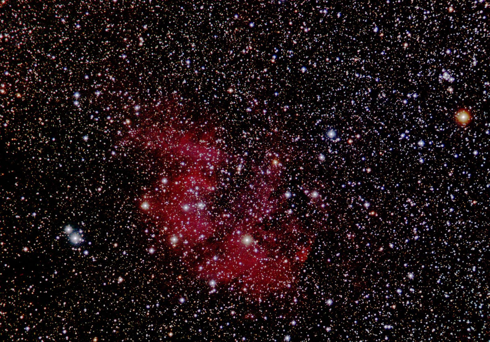
Figure 5. Color composite image of the nebula Sharpless 132 created using regular broad-band Red, Green and Blue Master Light Images.
What is needed is a way to bring out the nebula without bringing out the stars. This is what hybrid images can do. Another set of images was acquired for this target. In this case, 90-second (1.5 min) images in the Red, Green and Blue spectral bands were acquired. In addition, 900-second (15 min) images were acquired in Hα. Nebulas like Sharpless 132 emit predominantly in the Hα spectral band, so it was not necessary to also acquire Hβ and OIII narrow-band images. Master Red, Green, Blue and Hα images were created using Basic FITS Image Processing, Part I. A hybrid Red image was then created from the broad-band Red image and the Hα image as described in the first part of this webpage.
To create this hybrid image, photon flux densities for corresponding stars in the broad-band Red and narrow-band Hα Master Light images were measured using the Single Star Photometry Tool in AIP4WinV2. Figure 6 shows the average ratio of photon fluxes from stars in Hα images of various exposure times (90 to 900 seconds) to the photon fluxes of stars in a 90-second broad-band Red image. Data for constructing this graph were acquired from a separate imaging session. As this graph shows, the brightness of stars in Hα images is normally much less than the brightness of stars in broad-band Red images. In fact, it would take a Hα image with an exposure of almost 30 minutes to have stars as bright as those in a 90-second (1.5 min) broad-band Red image.
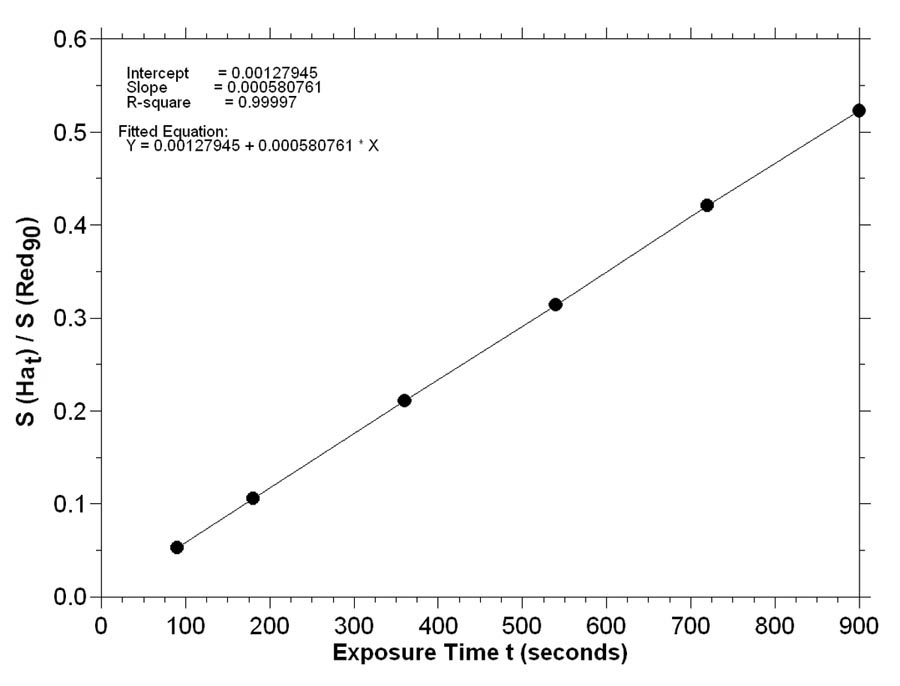
Figure 6. Ratio of photon fluxes from stars in Hα images of various exposure times to the photon flux of stars in a 90-second broad-band Red image.
For the imagery of Sharpless 132, the average ratio of photon fluxes from stars in the 900-second Hα Master Light Image to the photon fluxes of stars in the 90-second broad-band Red Master Light Image was 0.532. Thus, pixel values in the Hα Master Light Image were multiplied by 2 to bring the brightness of stars in that image close to that of stars in the Red Master Light Image. The two Master Light Images were then combined using the maximizing function in Maxim DL as described in the first part of this webpage. The resulting Hybrid Red Master Light Image was composited with the broad-band Green and Blue Master Light Images using Basic FITS Image Processing, Part III to create a color composite image. This color image was then contrast-stretched to bring out the nebula. The result is presented in Figure 7.
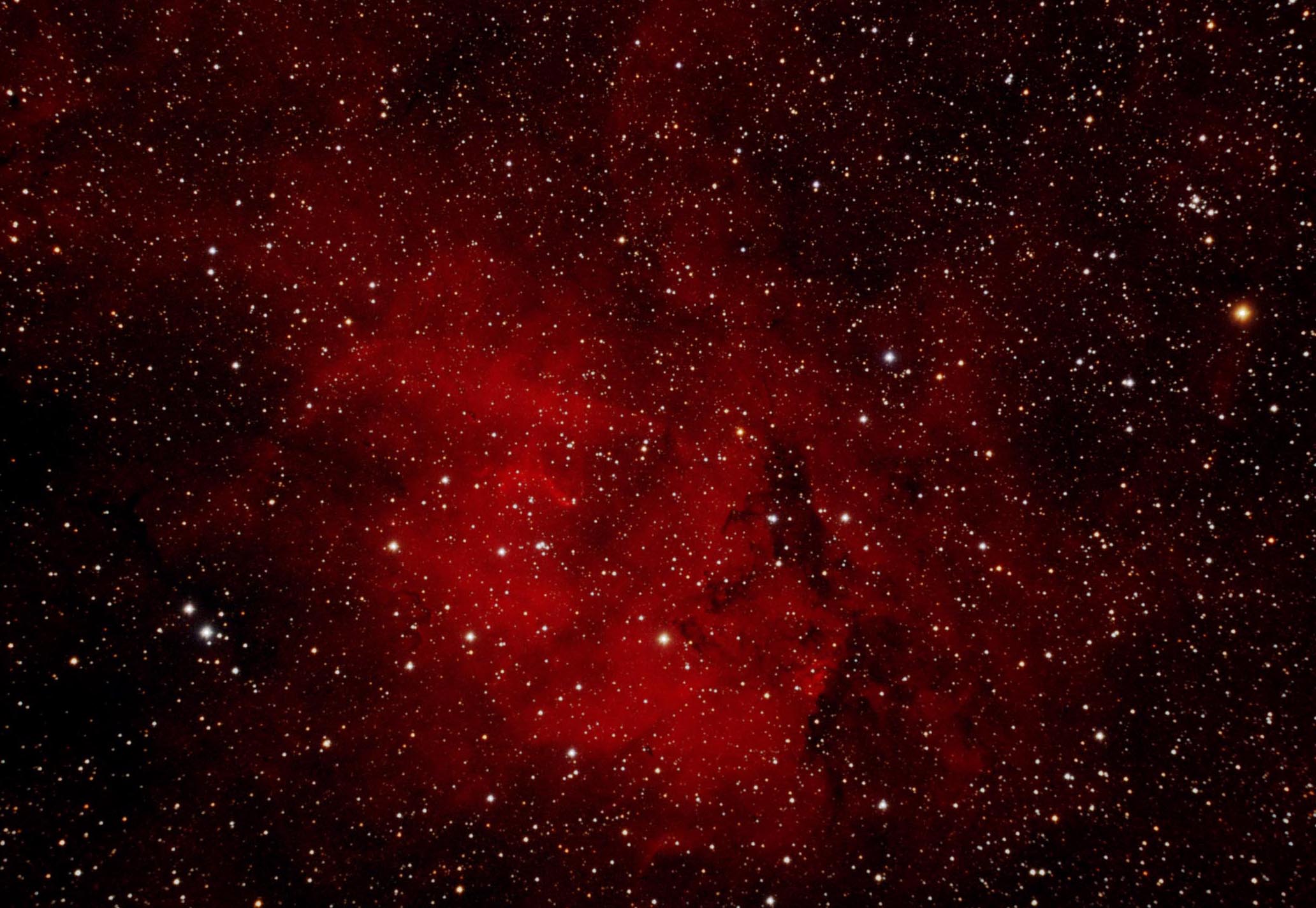
Figure 7. Color composite image of Sharpless 132 created using broad-band Green and Blue Images and a Hybrid Red Image.
Figure 7 is a big improvement over Figure 5. In Figure 7, the stars come from the 90-second broad-band Red, Green and Blue images while the nebula comes from the 900-second narrow-band Hα images. This color composite image did not need as much contrast-stretching since the nebula in the hybrid Red image was much brighter than in the regular broad-band Red image. Thus, the brightness of the stars in the color composite are maintained at an attractive level while the nebula is brought out. Also, using this procedure maintains the correct color balance among the stars and nebula (i.e., Figure 7 is a "true color" image like Figure 5).
Summary
The procedure outlined on this page appears to be an effective, objective method for combining broad-band and narrow-band images of astronomical objects, particularly emission nebulas. While its use is questionable for bright emission nebulas that can be adequately captured in regular broad-band Red, Green and Blue imagery (I think the color composite image on the right side of Figure 4 is fine), it should be useful for bringing out dimmer emission nebulas while maintaining attractive (properly exposed, not over-exposed) surrounding star fields. I'm still in the process of refining and testing this procedure. Changes and updates to the procedure will be included in future versions of this page.
 Return to SOCO Image Processing Page
Return to SOCO Main Page
Return to SOCO Image Processing Page
Return to SOCO Main Page
Questions or comments? Email SOCO@cat-star.org